4.4 Application

The use of our methodology is illustrated on smart meter energy usage for a sample of customers from SGSC consumer trial data which was available through Department of the Environment and Energy and Data61 CSIRO. It contains half-hourly general supply in KwH for 13,735 customers, resulting in 344,518,791 observations in total. The raw data for these consumers is of unequal length, with varying start and finish dates. Because our proposed methods evaluate probability distributions rather than raw data, neither of these data features would pose any threat to our methodology unless they contained any structure or systematic patterns. Additionally, there were missing values in the database but further investigation revealed that there is no structure in the missingness (see Supplementary paper for raw data features and missingness).

Clustering huge data sets presents a slew of difficulties. As a result, we dissect the larger problem and test our solutions on a small sample of prototype customers. To do this, data is first filtered to generate a clean sample, and then significant cyclic granularities (variables) for them are chosen. This is described in Section . The clean set is subsequently subsampled along all dimensions of interest, to ensure that the sampled data reveals some patterns across at least one specified variable, which is described in Section . By grouping the prototypes using our methods in Section and assessing their meaning, the study hopes to unravel some of the heterogeneities observed in energy usage data. Because our application does not employ additional customer data, we cannot explain why consumption varies, but rather try to identify how it varies.

4.4.1 Data filtering and variable selection

Choose a smaller subset of randomly selected $600$ customers with no implicit missing values for 2013.
Obtain $wpd$ for all cyclic granularities considered for these customers. It was found that hod (hour-of-day), moy (month-of-year) and wkndwday (weekend/weekday) are turning out to be significant for most customers. We use these three granularities while clustering.
Remove customers whose data for an entire category of hod, moy or wnwd is empty. For example, a customer who does not have data for an entire month is excluded because their monthly behavior cannot be analyzed.
Remove customers whose energy consumption is 0 in all deciles. These are the clients whose consumption is likely to remain essentially flat and with no intriguing repeated patterns that we are interested in studying.

4.4.2 Prototype selection

Supervised learning uses a training set of known information to categorize new events through instance selection. Instance selection (Olvera-López et al. (2010)) is a method of rejecting instances that are not helpful for classification. This is analogous to subsampling the population along all dimensions of interest such that the sampled data represents the primary features of the underlying distribution. Instance selection in unsupervised learning has received little attention in the literature. However, it could be a useful tool for evaluating model or method performance. There are several ways to approach prototype selection. Following the idea of Fan et al. (2021) of picking related examples (neighbors) for each instance (anchor), we can first use any dimensionality reduction techniques like MDS or PCA to project the data into a 2D space. Then pick a few “anchor” customers far apart in 2D space and pick a few neighbors for each. Unfortunately, this does not ensure that consumers with significant patterns across all variables are chosen. Tours can reveal variable separation that gets hidden in a single variable display better than static projections. Hence, we perform a linked tour with a t-SNE layout using the R package liminal (Lee (2021)) to identify customers who are more likely to have distinct patterns across the variables studied. (Refer to the supplementary article for further details). Figure shows the distribution across hod, moy and wnwd for the set of chosen $24$ customers that were chosen. The customers are split into batches of $12$ in (a) and (b). Each row in (a) and that in (b) represents the profile of one customer across different variables.

4.4.3 Clustering

The $24$ prototypes are clustered using the methodology described in Section and results are reported below. In the following plots, the median is shown by a line, and the shaded region shows the area between the $25^{th}$ and $75^{th}$ percentiles. Groups are colored differently whenever they represent different groupings. While plotting the clusters, RS-based scaling is applied to each customer, so that no customer dominates the shape of the summarized clusters because of magnitude. The plotting scales are not displayed since we want to emphasize comparable patterns rather than scales. The idea is that a customer in a cluster may have low total energy usage, but their behavior may be quite similar to a customer with high usage with respect to distributional pattern or significance across cyclic granularities.

4.4.3.1 JS-based distances

The $sindex$ is plotted against the number of clusters for clustering based on JS-based (JS-NQT) distances in Figure . The $sindex$ falls from around $0.56$ when $k=3$ to $0.54$ when $k$ increases. In our study, we use $k=4, 5$. Figure depicts the summarized distributions across $4$ and $5$ clusters in (a) and (b) respectively, and assists in characterizing each cluster. A-2, Groups A-3, and A-4 have profiles that correspond to B-2, B-3, and B-5, respectively. B-2 (id: 4-9 in Figure ) and B-5 (id: 21-24) have a hod pattern with a typical morning and evening peak, whereas the other groups have no distinct pattern or high variability throughout the day. A-1 is subdivided into B-1 and B-4, each of which has a distinct shape across moy and wnwd. B-4 (id: 16-20) is distinguished by higher energy consumption in the first few months of the year and greater variability in weekend usage. B-1 (id: 1-3) has higher consumption in the middle of the year (winter months) and a similar weekday-weekend inter-quartile range. When $k = 4$ is used, these two groups merge to form A-1, which has a moy profile of higher usage in both the beginning and middle of the year, which is not representative of the individuals. It may be worthwhile to compare Figures and to see if the summarized distributions across groups accurately characterized the groupings. If it has, then the majority of the members of the group should have a similar profile.

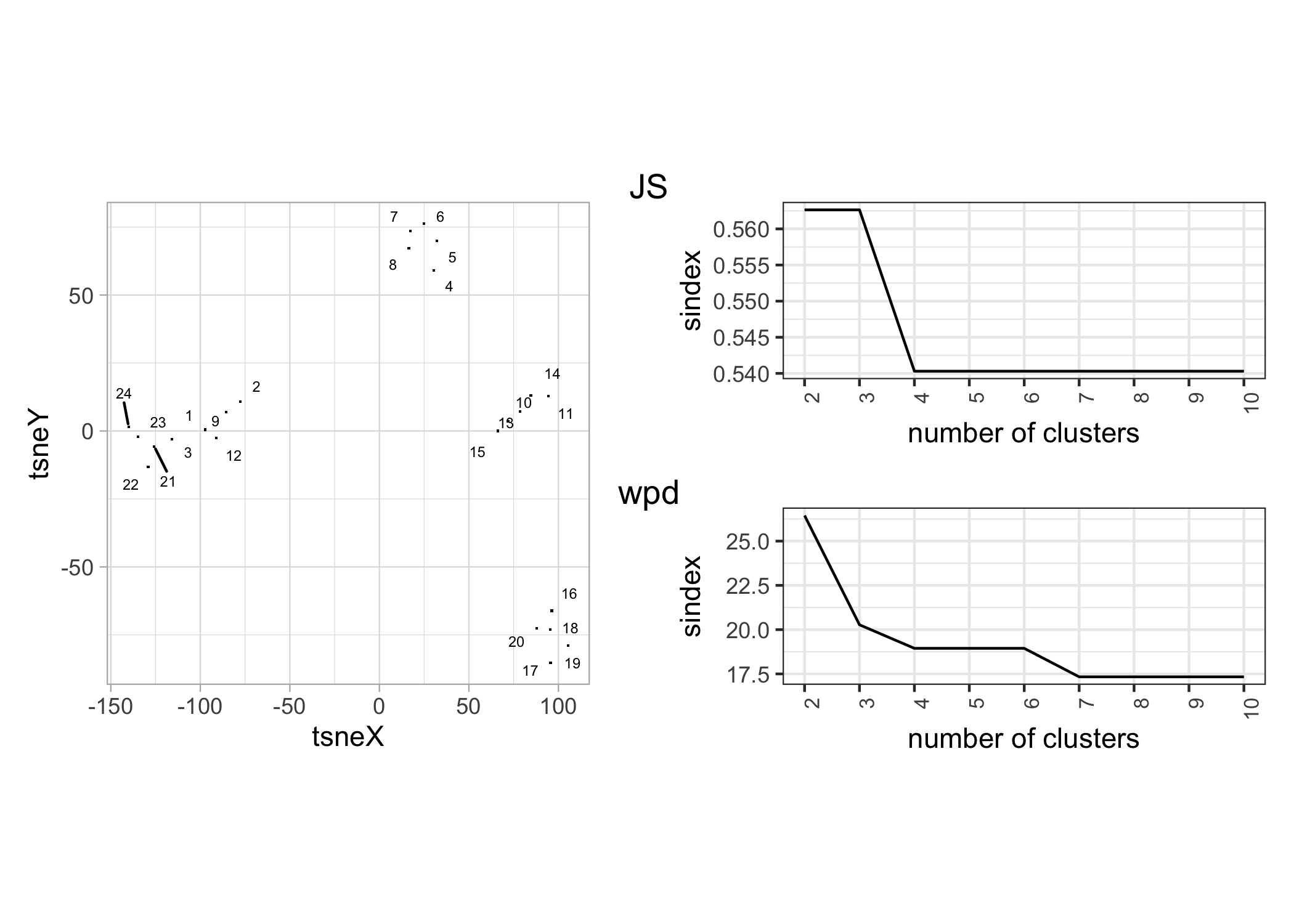
(a) shows t-SNE summary of the $24$ selected customers chosen through prototype selection, (b) and (c) shows a plot of sindex for different cluster size for clustering based on JS-based distances and wpd-distances respectively. The plot suggests optimal number of clusters as $4$ and $7$ respectively.

Figure 4.8: (a) shows t-SNE summary of the $24$ selected customers chosen through prototype selection, (b) and (c) shows a plot of sindex for different cluster size for clustering based on JS-based distances and wpd-distances respectively. The plot suggests optimal number of clusters as $4$ and $7$ respectively.

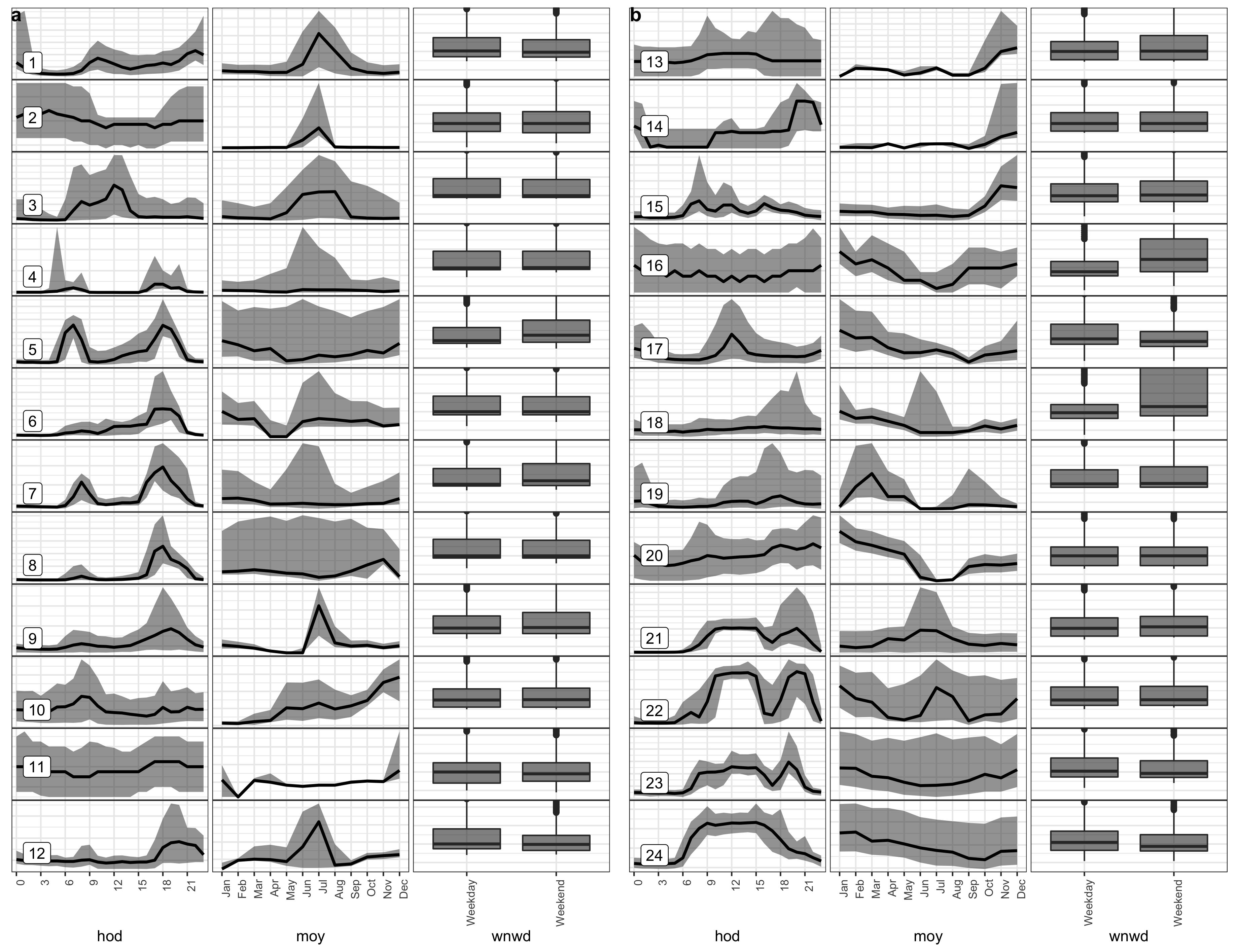
Figure 4.9: The distribution of electricity demand across individual customers over multiple granularities hod, moy, and wnwd are shown for the $24$ selected customers using quantile and box plots. They are split into batches of $12$ in (a) and (b), with each row in (a) or (b) representing a customer. Each customer is identified by their profile across all the granularities. A few of these customers have similar distributions across moy and some are similar in their hod distributions. Distributional differences across categories of wnwd are not discernable except for a couple of customers (id: 16 and 18).

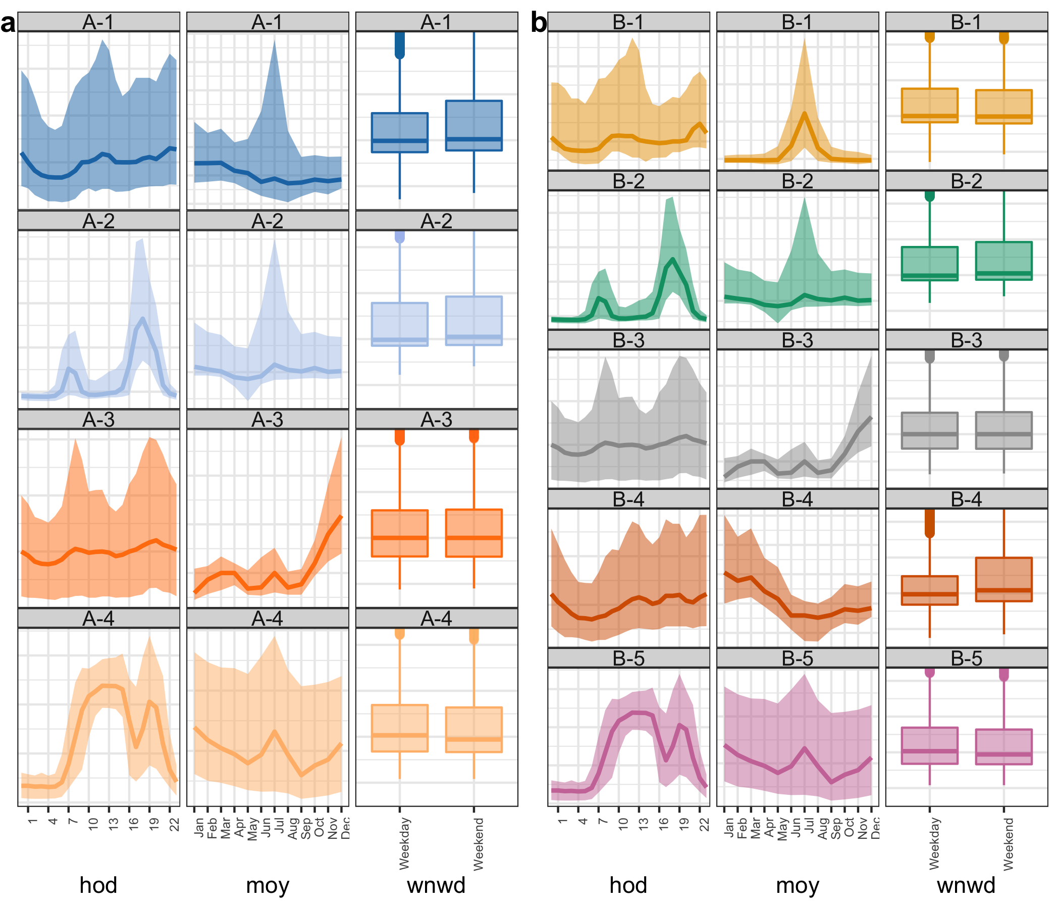
Figure 4.10: For $k = 4$ (a) and $k=5$ (b), the distribution of electricity demand across groups over hod, moy, and wnwd is shown. Groups A-2, A-3, and A-4 profiles correspond to Groups B-2, B-3, and B-5, respectively. A-1 is split into B-1 and B-4, each of which has a distinct shape across moy and wnwd. B-4 (id: 16-20) is characterized by higher energy consumption in the first few months of the year and more variation in weekend usage. B-1 (id:1-3) is distinguished by higher consumption in the middle of the year (winter months) and similar weekday-weekend inter-quartile range. When $k = 4$ is used, these two groups merge to form A-1, which has a moy profile of higher usage in both the beginning and middle of the year, which is not representative of the individuals in the group.

4.4.3.2 wpd-based distances

In Figure , the $sindex$ is plotted against the number of clusters for clustering based on wpd-based distances. The scales are very different from those used in JS-based clustering. The $sindex$ falls from around $20$ when $k=3$ to $19$ when $k=4$ and further decreases to $17.5$ with $k>7$. Thus, there are few choices available for the number of clusters. The groupings with $k=4$ is shown through a parallel coordinate plot with the three significant cyclic granularities. The variables are sorted according to their separation across classes (rather than their overall variation between classes). This means that $moy$ is the most important variable in distinguishing the groups, followed by $hod$ and $wnwd$. The two customers (id: 16 and 18) that have significant differences between $wnwd$ categories (in Figure ) stand out from the rest of the customers. Group-4 has a higher $wpd$ for hod than moy or wkndwday. Group-2 and Group-3 have the most distinct patterns across moy. Group-1 is a mixed group that has strong patterns on at least one of the three variables. When $k=3$ is used, Group-2 and Group-3 are merged because their patterns relative to moy, hod and wnwd are the same. The findings vary from JS-based clustering, yet it is a helpful grouping.

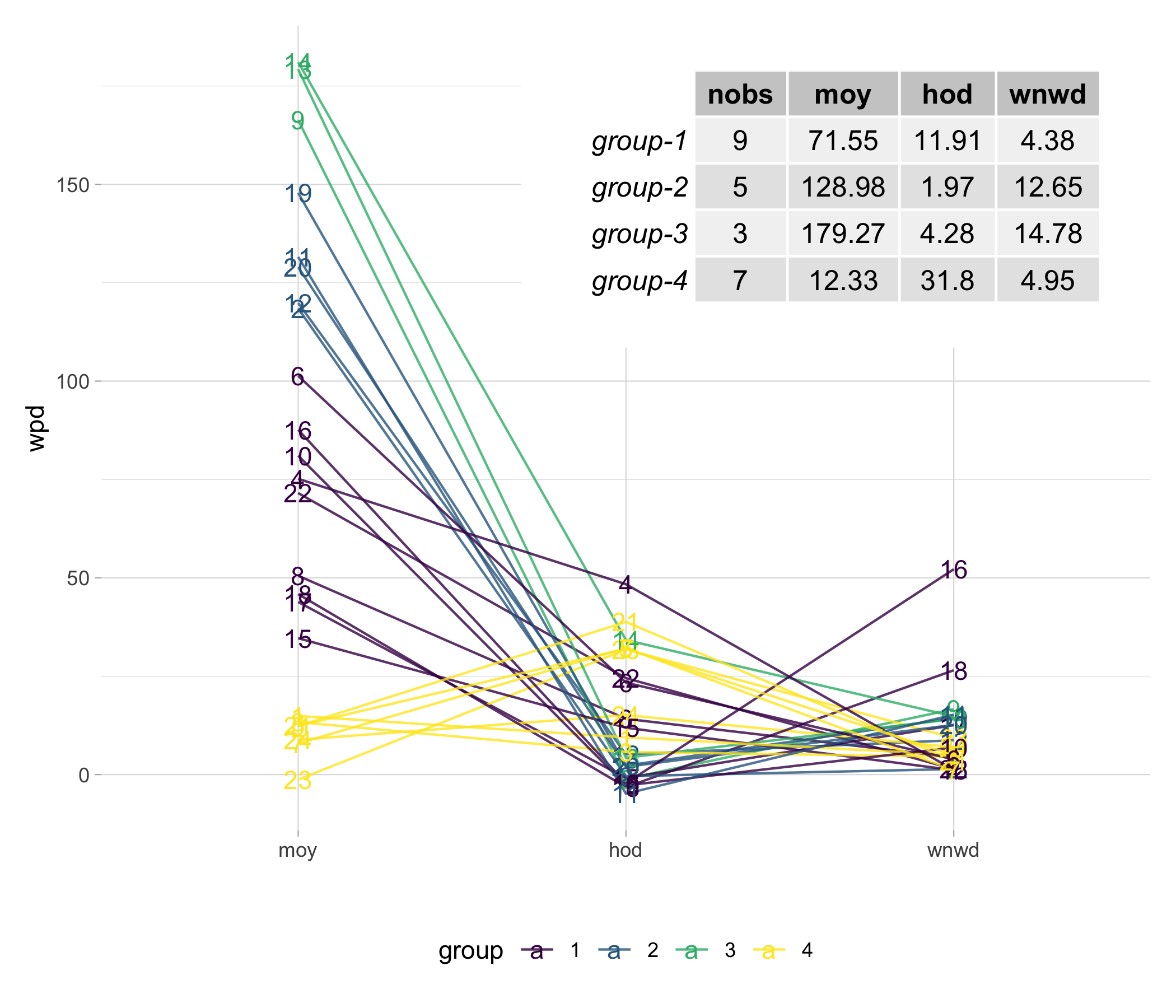
Each of the $24$ customers is represented by a parallel coordinate plot (a) with four wpd-based groupings. Plot (b) which shows median $wpd$ values for each group. The plot shows that moy is the most important variable in identifying clusters, whereas wnwd is the least significant and has the least fluctuation. Two customers (id: 16 and 18) with high $wpd$ across wnwd stand out in this display. Group-4 has a higher $wpd$ for hod than moy or wnwd. Group-2 and Group-3 have the most discernible pattern across moy. Group-1 is a mixed group with strong patterns across at least one of the three variables. All of these could be observed from the plot or the table (b).

Figure 4.11: Each of the $24$ customers is represented by a parallel coordinate plot (a) with four wpd-based groupings. Plot (b) which shows median $wpd$ values for each group. The plot shows that moy is the most important variable in identifying clusters, whereas wnwd is the least significant and has the least fluctuation. Two customers (id: 16 and 18) with high $wpd$ across wnwd stand out in this display. Group-4 has a higher $wpd$ for hod than moy or wnwd. Group-2 and Group-3 have the most discernible pattern across moy. Group-1 is a mixed group with strong patterns across at least one of the three variables. All of these could be observed from the plot or the table (b).

Things become far more complicated when we consider a larger data set with more uncertainty, as they do with any clustering problem. Summarizing distributions across clusters with varied or outlying customers can result in a shape that does not represent the group. Furthermore, combining heterogeneous customers may result in similar-looking final clusters that are not effective for visually differentiating them. It is also worth noting that the weekend/weekday behavior in the given case does not characterize most selected customers. This, however, will not be true for all of the customers in the data set. If more extensive prototype selection is used, resulting in more comprehensive prototypes in the data set, this method might be used to classify the entire data set into these prototype behaviors. However, the goal of this section was to have a few customers that have significant patterns over one or more cyclic granularities, apply our methodology to cluster them, and demonstrate that the method produces useful clusters.