3.4 Application to residential smart meter dataset

The smart meter data set for eight households in Melbourne was procured by downloading the data from the energy supplier/retailer. The data has been cleaned to form a tsibble (Wang, Cook, and Hyndman 2020a) containing half-hourly electricity consumption from July to December 2019 for each of the households. No behavioral pattern is likely to be discerned from the time plot of energy usage over the entire period, since the plot will have too many observations squeezed in a linear representation. When we zoom into the September 2019 data in Figure (b), some patterns are visible in terms of peaks and troughs, but we do not know if they are regular or what is their period.

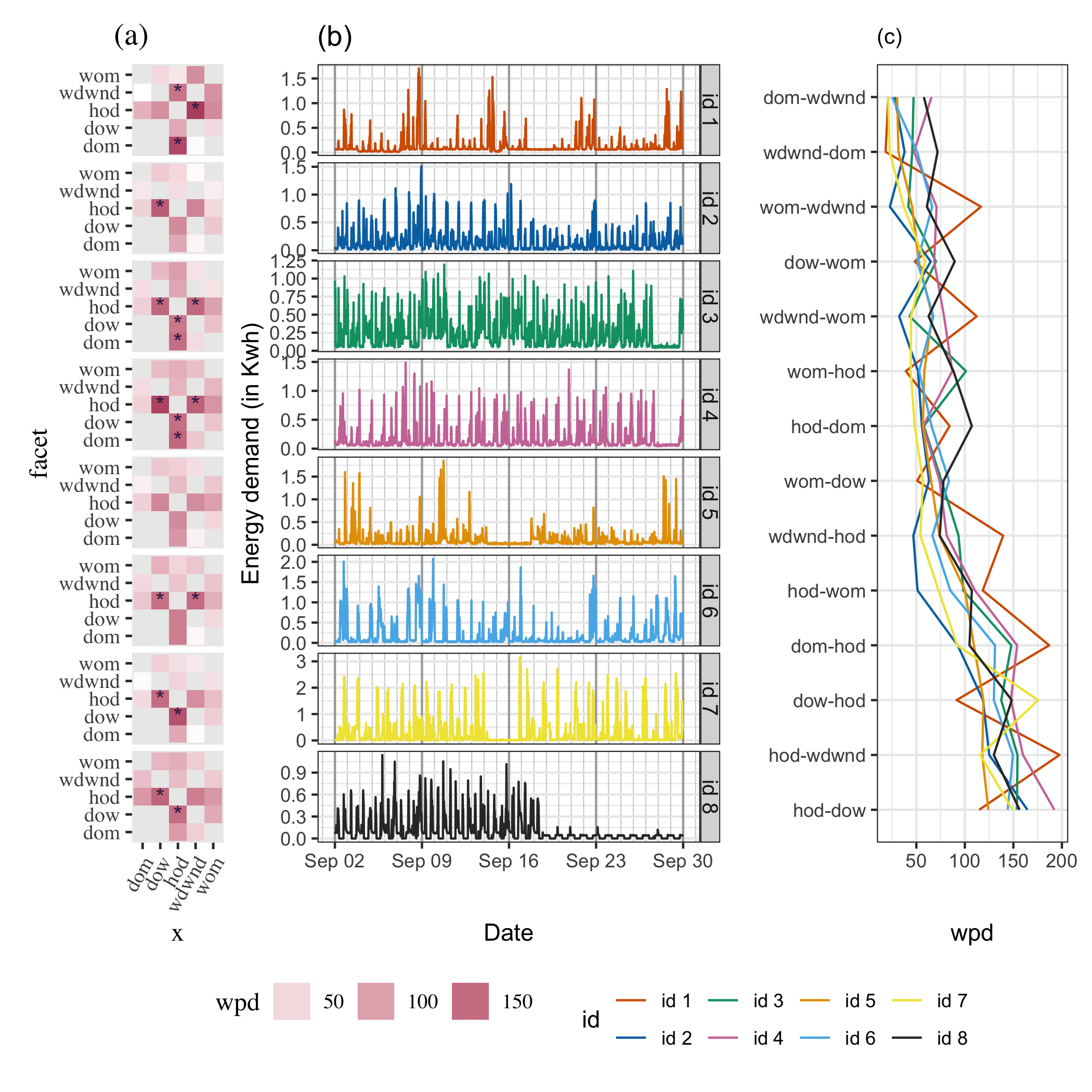
Figure 3.7: An ensemble plot with a heatmap (a), line plot (b), parallel coordinate plot (c) to demonstrate energy behavior of the households in different ways. Panel (b) shows the raw demand series for September to highlight the repetitive patterns of energy demand. Panel (a) shows \(\wpd\) values across harmonies where a darker color indicates a higher ranking harmony. A significant harmony is shown with an asterisk. For example, ids 7 and 8 have significant patterns across (hod, dow) and (dow, hod). Panel (c) is useful for comparing households across harmonies. For example, for the harmony (dow-hod), ids 1 and 7 have the least and highest \(\wpd\) respectively.

Electricity demand, in general, has daily, weekly and annual seasonal patterns. However, it is not apparent from this view if all households have those patterns, or how strong they are in each case. It is also not clear from this view if any other periodic patterns are present in any household. We start the analysis by choosing a few harmonies, and ranking them for each of these households. The ranking and selection of significant harmonies is validated by analyzing the distribution of energy usage across significant harmonies.

Choosing cyclic granularities of interest and removing clashes

Let \(v_{i, t}\) denote the electricity demand for the \(i^{th}\) household in time period \(t\). The series \(\{v_{i, 1},\dots,v_{i,T}\}\) is the linear granularity corresponding to half-hour since the interval of the tsibble is 30 minutes. We consider coarser linear granularities like hour, day, week and month from the commonly used Gregorian calendar. From the four linear granularities of hour, day, week, and month, we obtain \(N_C = 4\times 3/2 = 6\) cyclic granularities: “hour_day,” “hour_week,” “hour_month,” “day_ week,” “day_month” and “week_month.” Further, we add cyclic granularity day-type (“wknd wday”) to capture weekend and weekday behavior. Thus, seven cyclic granularities are considered to be of interest. The pairs of cyclic granularities (\(C_{N_C}\)) will have \(7\times 6=42\) elements. The set of possible harmonies \(H_{N_C}\) from \(C_{N_C}\) are chosen by removing clashes using procedures described in Gupta et al. (2021). Table shows \(14\) harmony pairs that belong to \(H_{N_C}\).

Table 3.2: Ranking of harmonies for the eight households with significance marked for different thresholds. Rankings are different and at most three harmonies are significant for any household. The number of harmonies to explore is reduced from 42 to 3.

facet variable	x variable	id 1	id 2	id 3	id 4	id 5	id 6	id 7	id 8
hod	wdwnd	1	2	1	2	3	1	3	3
dom	hod	2	4	3	3	4	3	4	6
wdwnd	hod	3	10	7	7	6	8	8	10
hod	wom	4	9	6	5	5	5	5	5
wom	wdwnd	5	14	14	10	12	9	12	13
hod	dow	6	1	2	1	1	2	2	1
wdwnd	wom	7	12	13	8	7	7	10	12
dow	hod	8	3	4	4	2	4	1	2
hod	dom	9	7	10	13	10	10	9	4
wom	dow	10	6	8	9	8	6	7	9
dow	wom	11	5	9	11	11	12	6	7
wom	hod	12	8	5	6	9	11	11	8
dom	wdwnd	13	13	11	12	14	14	14	14
wdwnd	dom	14	11	12	14	13	13	13	11

Selecting and ranking harmonies for all households

\(\wpd_{i}\) is computed on \(v_{i, t}\) for all harmony pairs \(\in H_{N_C}\) and for each household \(i \in \{1, 2, \dots, 8\}\). The harmony pairs are then arranged in descending order and highlighted with ***, ** and * corresponding to the \(99^{th}\), \(95^{th}\) and \(90^{th}\) percentile threshold. Table shows the rank of the harmonies for different households. The rankings are different for different households, which is a reflection of their varied behaviors. Most importantly, there are at most three harmonies that are significant for any household. This is a huge reduction in the number of potential harmonies to explore.

Detecting patterns not apparent from linear display

Figure helps to compare households through the heatmap (a) across harmony pairs. Here dom, dow, wdwnd are abbreviations for day-of-month, day-of-week, weekday/weekend and so on. The colors represent the value of \(\wpd\). Darker cells correspond to higher values of \(\wpd\). Those with * correspond to \(\wpd\) values above \(\wpdsub{threshold95}\).

We can now see some patterns that were not discernible in Panel (b), including:

1. id 7 and 8 have the same significant harmonies despite having very different total energy usage.
2. id 6 and 7 differ in the sense that for id 6, the difference in patterns is only during weekday/weekends, whereas for id 7 all or few other days of the week are also important. This might be due to their flexible work routines or different day-off.
3. There are no significant periodic patterns for id 5 when we fix the threshold to \(\wpdsub{threshold95}\).

Note that the \(\wpd\) values are computed over the entire range, but the linear display in (b) is only for September, with the major and minor x-axis corresponding to weeks and days respectively.

Comparing households and validating rank of harmonies

According to Figure (c), for the harmony pair (dow-hod), household id 7 has the greatest value of \(\wpd\), while id 1 has the least. From Table it can be seen that the harmony pair (dow, hod) is important for id 7; however, it has been labeled as an inconsequential pair for id 1. The distribution of energy demand for both of these households, with dow as the facet and hod on the x-axis, may help explain the choice. Figure demonstrates that for id 7, the median (black) and quartile deviation (orange) of energy consumption fluctuates for most hours of the day and days of the week, while for id 1, daily patterns are more consistent within weekdays and weekends. As a result, for id 1, it is more appropriate to examine the distributional difference solely across (dow, wdwnd), which has been rated higher in Table .

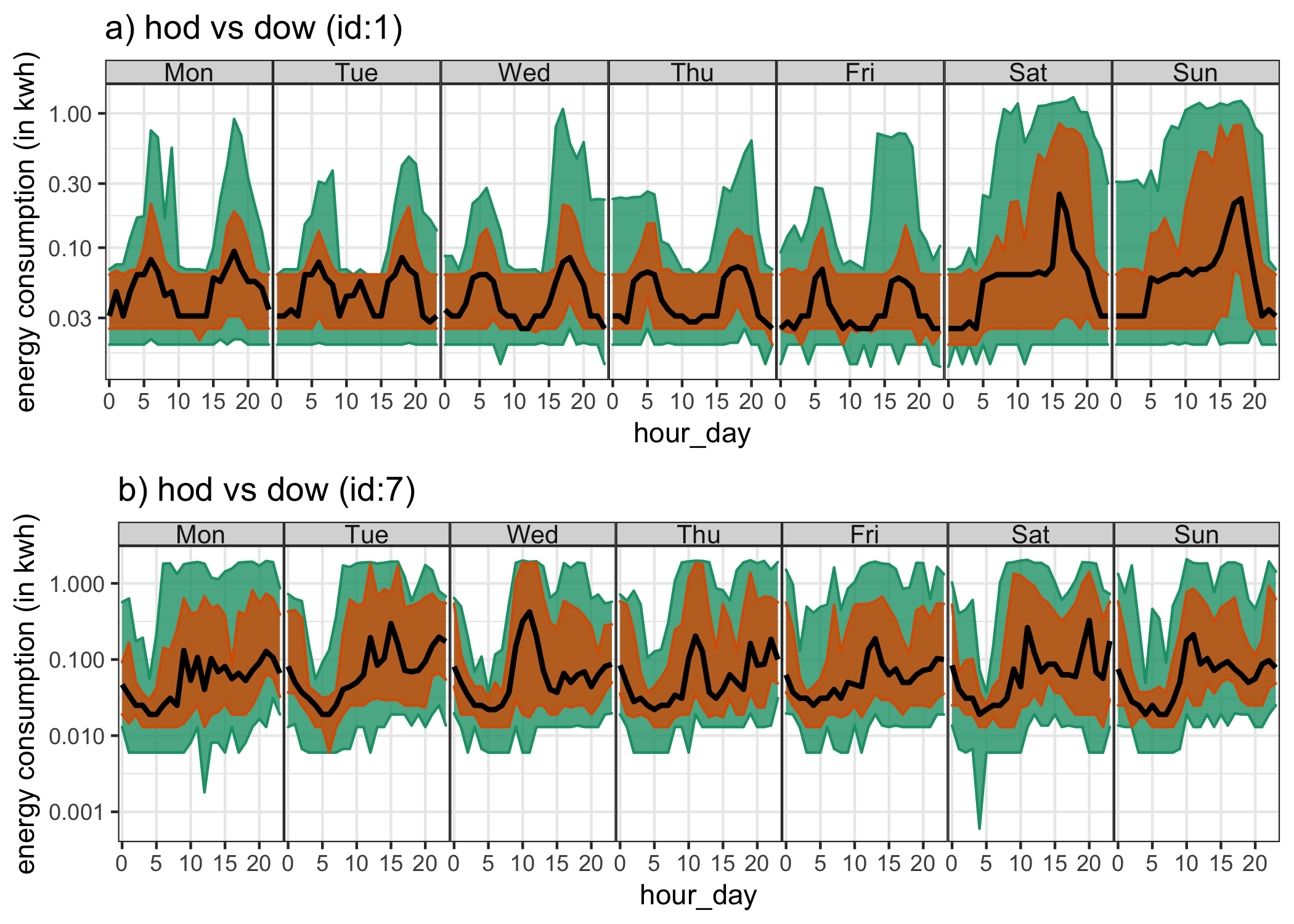
Figure 3.8: Comparing distribution of energy demand shown for household id 1 (a) and 7 (b) across hod in x-axis and dow in facets through quantile area plots. The value of \(\wpd\) in Table 3 suggests that the harmony pair (dow, hod) is significant for household id 7, but not for id 1. This implies that distributional differences are captured more by this harmony for id 7, which is apparent from this display with more fluctuations across median and 75th percentile for different hours of the day and day of week. For id 1, patterns look similar within weekdays and weekends. Here, the median is represented by the black line, the orange area corresponds to quartile deviation and the green area corresponds to area between \(10^{th}\) and \(90^{th}\) quantile.