3.3 Ranking and selection of cyclic granularities

A cyclic granularity is referred to as “significant” if there is a significant distributional difference of the measured variable between different categories of the harmony. In this section, a selection criterion to choose significant harmonies is provided, thereby eliminating all harmonies that exhibit non-significant differences in the measured variable. The distance measure $\wpd$ is used as a test statistic to test the null hypothesis that no harmony/cyclic granularity is significant. We select only those harmonies/cyclic granularities for which the test fails. They are then ranked based on how well they capture variation in the measured variable.

3.3.1 Selection

A threshold (and consequently a selection criterion) is chosen using the notion of randomization tests (Edgington and Onghena 2007). The data is permuted several times and $\wpd$ is computed for each of the permuted data sets to obtain the sampling distribution of $\wpd$ under the null hypothesis. If the null hypothesis is true, then $\wpd$ obtained from the original data set would be a likely value in the sampling distribution. But in case the null hypothesis is not true, then it is less probable that $\wpd$ obtained for the original data will be from the same distribution. This idea is utilized to come up with a threshold for selection, denoted by $\wpdsub{threshold}$, defined as the $99^{th}$ percentile of the sampling distribution. A harmony is selected if the value of $\wpd$ for that harmony is greater than the chosen threshold. The detailed algorithm for choosing a threshold and selection procedure (for two cyclic granularities) is listed as follows:

Input: All harmonies of the form $\{(A, B),~ A = \{ a_j: j = 1, 2, \dots, \nx\},~ B = \{ b_k: k = 1, 2, \dots, \nf\}\}$, $\forall (A, B) \in H_{N_C}$.
Output: Harmony pairs $(A, B)$ for which $\wpd$ is significant.

For each harmony pair $(A, B) \in H_{N_C}$, the following steps are taken.
1. Given the measured variable; $\{v_t: t=0, 1, 2, \dots, T-1\}$, $\wpd$ is computed and is represented by $\wpd^{A, B}_{obs}$.
2. For $i=1,\dots,m$, randomly permute the original time series: $\{v_t^{i}: t=0, 1, 2, \dots, T-1\}$ and compute $\wpd^{A, B}_{i}$ from $\{v_t^{i}\}$.
3. Define $\wpdsub{sample} = \{\wpd^{A, B}_{1}, \dots, \wpd^{A, B}_{M}\}$.
Stack the $\wpdsub{sample}$ vectors as $\wpdsub{sample}^{\text{all}}$ and compute its $p = 100(1-\alpha)$ percentiles as $\wpdsub{threshold\emph{p}}$.
If $\wpd^{A, B}_{obs} > \wpdsub{threshold\emph{p}}$, harmony pair $(A, B)$ is selected at the $1-p/100$ level, otherwise rejected.
Harmonies selected using the $99^{th}$, $95^{th}$ and $90^{th}$ thresholds are tagged as ***, **, * respectively.

3.3.2 Ranking

The distribution of $\wpd$ is expected to be similar for all harmonies under the null hypothesis, since they have been adjusted for different number of categories for the harmonies or underlying distribution of the measured variable. Hence, the values of $\wpd$ for different harmonies are comparable and can be used to rank the significant harmonies. A higher value of $\wpd$ for a harmony indicates that higher maximum variation in the measured variable is captured through that harmony.

Figure also presents the results of $\wpd$ from the illustrative designs in Section . The value of $\wpd$ under null design (a) is the least, followed by (b), (c) and (d). This aligns with the principle of $\wpd$, which is expected to have lowest value for null designs and highest for designs of the form $\Dfx$ (d). Moreover, note the relative differences in $\wpd$ values between (b) and (c). The value of the tuning parameter $\lambda$ is set to 2/3, which gives greater emphasis to differences in x-axis categories than facets.

Again consider (a) and (b) with a $\wpd$ value of 20.5 and 145 respectively. This is because there is a more gradual increase across hours of the day than across months of the year. If the order of categories is ignored, the resulting $\wpd$ values are $97.8$ and $161$ respectively, because differences between any hours of the day tend to be larger than differences only between consecutive hours. Similarly, Figures (a) and (b) have $\wpd$ values of $110.79$ and $125.82$ respectively. The ranking implies that the distributional differences are more prominent for the second household, as is also seen from the bigger fluctuations in the $90^{th}$ percentile than for the first household.

3.3.3 Simulations

Simulations were carried out to explore the behavior of $\wpd$ as $\nx$ and $\nf$ were varied, in order to compare and evaluate different normalization approaches. More detailed simulation results, including an exploration of the size and power of the proposed test, are contained in the supplements.

Simulation design

$m=1$

Observations were generated from a N(0,1) distribution for $\nx \in \{2, 3, 5, 7, 9, 14, 17, 20, 24, 31, 42, 50\}$, with $\nsub{times} = 500$ observations drawn for each combination of categories. This design corresponds to $\Dnull$. For each of the categories, there were $\nsub{sim}=200$ replications, so that the distribution of $\wpd$ under $\Dnull$ could be observed. Let $\wpd_{\ell, s}$ denote the value of $\wpd$ obtained for the $\ell^{th}$ panel and $s^{th}$ simulation.

$m=2$

Similarly, observations were generated from a N(0,1) distribution for each combination of $\nx$ and $\nf$ from $\{2, 3, 5, 7, 14, 20, 31, 50\}$, with $\nsub{times} = 500$ observations drawn for each of the $64$ combinations.

Results

Figure shows that both the location and scale of the distributions change across panels. This is not desirable under $\Dnull$ as it would mean comparisons of $\wpd$ values are not appropriate across different $\nx$ and $\nf$ values. Table gives the summary of a Gamma generalized linear model to capture the relationship between $\wpdsub{raw}$ and the number of comparisons. The intercepts and slopes are similar, independent of the underlying distributions (see supplementary paper for details) and hence the coefficients are shown for the case when observations are drawn from a N(0,1) distribution. Figure shows the distribution of $\wpdsub{perm}$ and $\wpdsub{glm-scaled}$ on the same scale to show that a combination approach could be used for higher values of $\nx$ and $\nf$ to alleviate the computational time of the permutation approach.

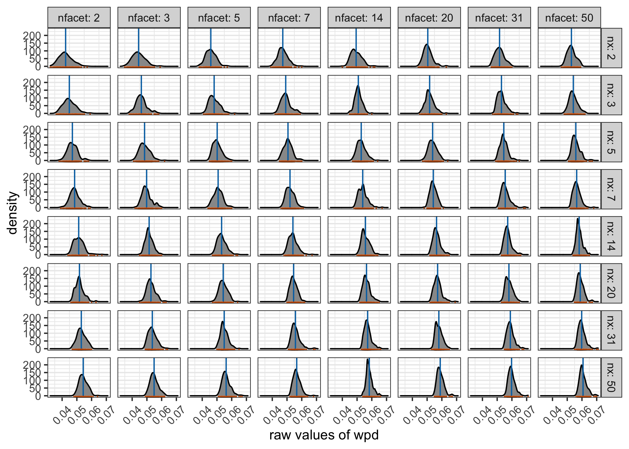
$Distribution of $\wpdsub{raw}$ is plotted across different $\nx$ and $\nf$ categories under $\Dnull$ through density and rug plots. Both location (blue line) and scale (orange marks) of the distribution shifts for different panels. This is not desirable since under the null design, the distribution is not expected to capture any differences.$

Figure 3.5: Distribution of $\wpdsub{raw}$ is plotted across different $\nx$ and $\nf$ categories under $\Dnull$ through density and rug plots. Both location (blue line) and scale (orange marks) of the distribution shifts for different panels. This is not desirable since under the null design, the distribution is not expected to capture any differences.

Table 3.1: Results of generalised linear model to capture the relationship between $\wpdsub{raw}$ and the number of comparisons.
$m$	term	estimate	std.error	statistic
1	Intercept	26.09	0.54	48.33
1	$\log(\nx \times \nf)$	-1.87	0.19	-9.89
2	Intercept	23.40	0.22	104.14
2	$\log(\nx \times \nf)$	-0.96	0.04	-21.75

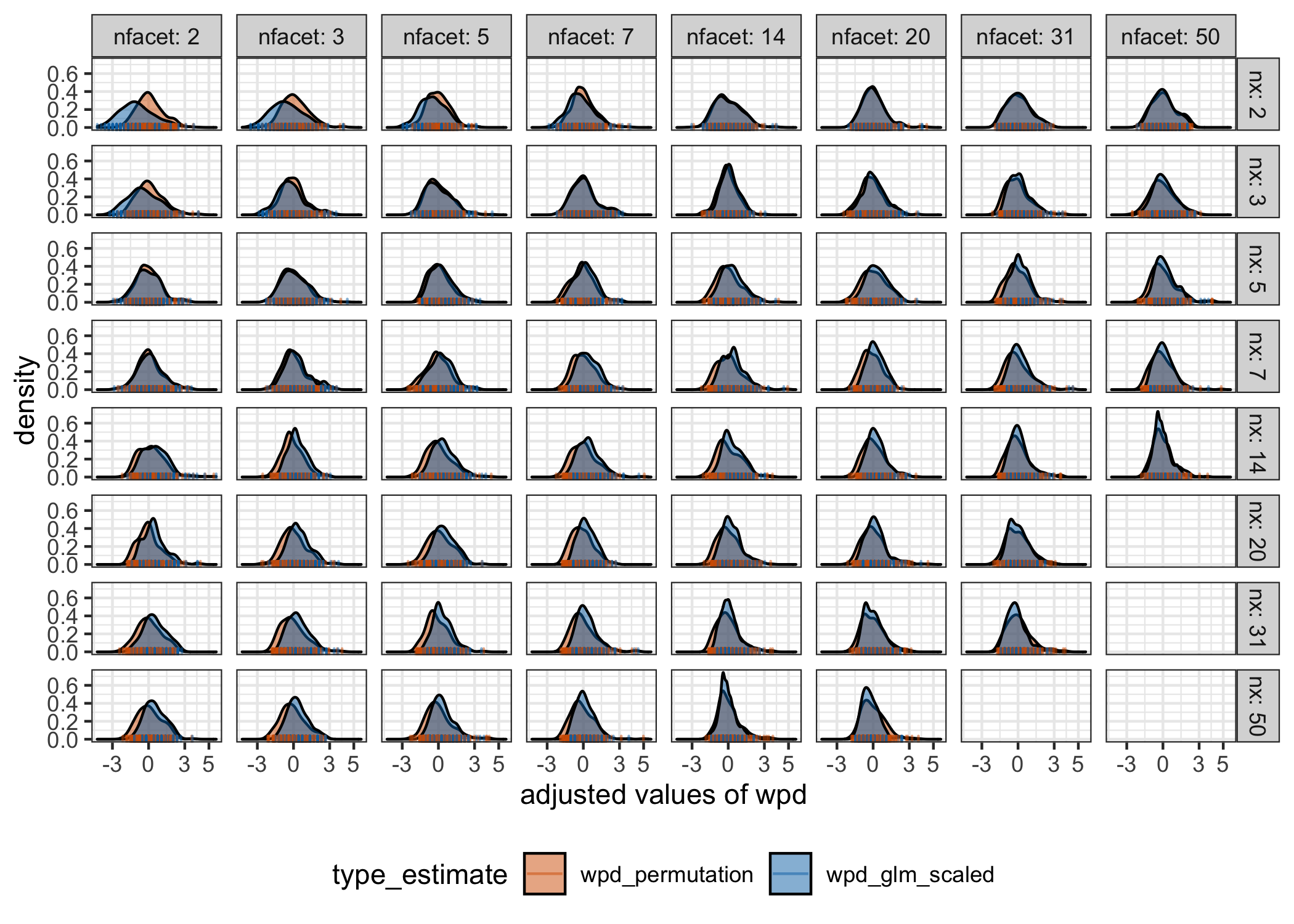
$The distributions of $\wpdsub{perm}$ and $\wpdsub{glm-scaled}$ are overlaid to compare the location and scale across different $\nx$ and $\nf$. $\wpdsub{norm}$ takes the value of $\wpdsub{perm}$ for lower levels, and $\wpdsub{glm-scaled}$ for higher levels to to alleviate the problem of computational time in permutation approaches. This is possible as the distribution of the adjusted measure looks similar for both approaches for higher levels.$

Figure 3.6: The distributions of $\wpdsub{perm}$ and $\wpdsub{glm-scaled}$ are overlaid to compare the location and scale across different $\nx$ and $\nf$. $\wpdsub{norm}$ takes the value of $\wpdsub{perm}$ for lower levels, and $\wpdsub{glm-scaled}$ for higher levels to to alleviate the problem of computational time in permutation approaches. This is possible as the distribution of the adjusted measure looks similar for both approaches for higher levels.

These results justify our use of the permutation approach when $\nx<5$ and $\nf<5$, and the use of the GLM otherwise.