3.2 Proposed distance measure
We propose a measure called Weighted Pairwise Distances (\(\wpd\)) to detect distributional differences in the measured variable across cyclic granularities.
3.2.1 Principle
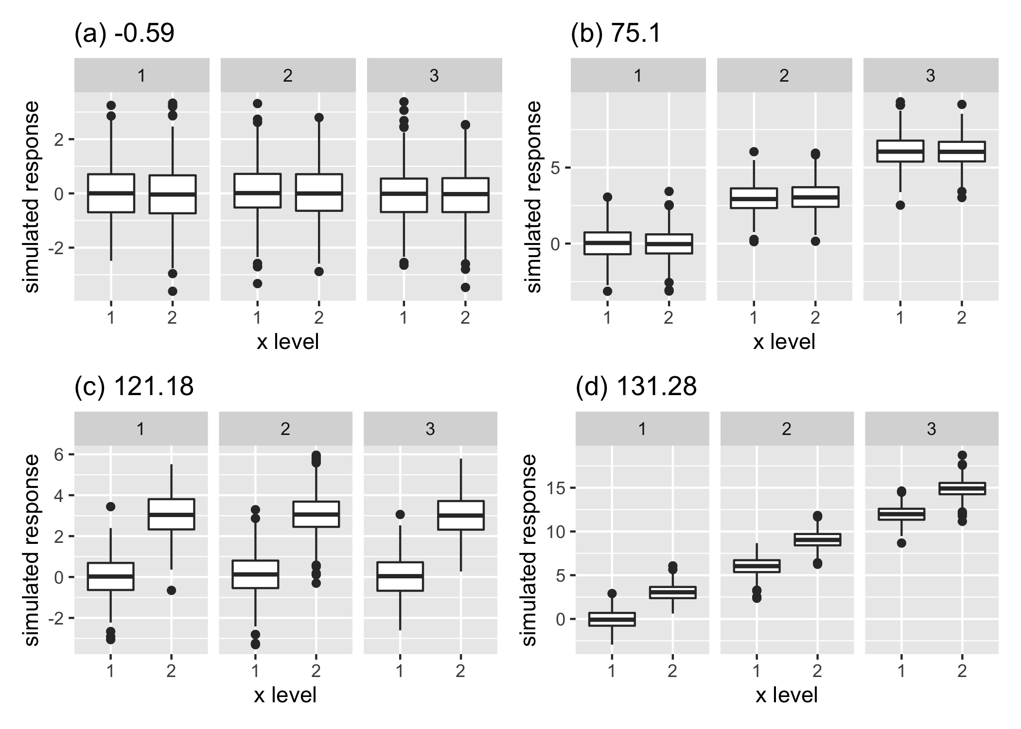
Figure 3.3: An example illustrating the principle of the proposed distance measure, displaying the distribution of a normally distributed variable in four panels each with two x-axis categories and three facet levels, but with different designs. Panel (a) is not interesting as the distribution of the variable does not depend on x or facet categories. Panels (b) and (c) are more interesting than (a) since there is a change in distribution either across facets (b) or x-axis (c). Panel (d) is most interesting in terms of capturing structure in the variable as the distribution of the variable changes across both facet and x-axis variable. The value of our proposed distance measure is presented for each panel, the relative differences between which will be explained later in Section 3.3.2.
The principle behind the construction of \(\wpd\) is explained through a simple example in Figure . Each of these figures describes a panel with two x-axis categories and three facet levels, but with different designs. Figure a has all categories drawn from a standard normal distribution for each facet. It is not a particularly interesting display, as the distributions do not vary across x-axis or facet categories. Figure b has x categories drawn from the same distribution, but across facets the distributions are three standard deviations apart. Figure c exhibits the opposite situation where distribution between the x-axis categories are three standard deviations apart, but they do not change across facets. In Figure d, the distribution varies across both facet and x-axis categories by three standard deviations.
If the panels are to be ranked in order of capturing maximum variation in the measured variable from minimum to maximum, then an obvious choice would be (a) followed by (b), (c) and then (d). It might be argued that it is not clear if (b) should precede or succeed (c) in the ranking. Gestalt theory suggests items placed at close proximity can be compared more easily, because people assume that they are in the same group and apart from other groups. With this principle in mind, Panel (b) is considered less informative compared to Panel (c) in emphasizing the distributional differences.
For displays showing a single cyclic granularity rather than pairs of granularities, we have only two design choices corresponding to no difference and significant differences between categories of that cyclic granularity.
The proposed measure \(\wpd\) is constructed in such a way that it can be used to rank panels of different designs as well as test if a design is interesting. This measure is aimed to be an estimate of the maximum variation in the measured variable explained by the panel. A higher value of \(\wpd\) would indicate that the panel is interesting to look at, whereas a lower value would indicate otherwise.
3.2.2 Notation
Let the number of cyclic granularities considered in the display be \(m\). The notations and methodology are described in detail for \(m=2\). But it can be easily extended to \(m>2\). Consider two cyclic granularities \(A\) and \(B\), such that \(A = \{a_j: j = 1, 2, \dots, \nx\}\) and \(B = \{b_k: k = 1, 2, \dots, \nf\}\) with \(A\) placed across the x-axis and \(B\) across facets. Let \(v = \{v_t: t = 0, 1, 2, \dots, T-1\}\) be a continuous variable observed across \(T\) time points. This data structure with \(\nx\) x-axis levels and \(\nf\) facet levels is referred to as a \((\nx, \nf)\) panel. For example, a \((2, 3)\) panel will have cyclic granularities with two x-axis levels and three facet levels. Let the four elementary designs as described in Figure be \(\Dnull\) (referred to as “null distribution”) where there is no difference in distribution of \(v\) for \(A\) or \(B\), \(\Df\) denotes the set of designs where there is difference in distribution of \(v\) for \(B\) and not for \(A\). Similarly, \(\Dx\) denotes the set of designs where difference is observed only across A. Finally, \(\Dfx\) denotes those designs for which difference is observed across both \(A\) and \(B\). We can consider a single granularity (\(m = 1\)) as a special case of two granularities with \(\nf = 1\).
3.2.3 Computation
The computation of the distance measure \(\wpd\) for a panel involves characterizing distributions, computing distances between distributions, choosing a tuning parameter to specify the weight for different groups of distances and summarizing those weighted distances appropriately to estimate maximum variation. Furthermore, the data needs to be appropriately transformed to ensure that the value of \(\wpd\) emphasizes detection of distributional differences across categories and not across different data generating processes.
Data transformation
The intended aim of \(\wpd\) is to capture differences in categories irrespective of the distribution from which the data is generated. Hence, as a pre-processing step, the raw data is normal-quantile transformed (NQT) (Krzysztofowicz 1997), so that the transformed data follows a standard normal distribution. The empirical NQT involves the following steps:
- The observations of measured variable \(v\) are sorted from the smallest to the largest observation \(v_{(1)},\dots, v_{(n)}\).
- The cumulative probabilities \(p_{(1)},\dots, p_{(n)}\) are estimated using \(p_{(i)} = i/(n + 1)\) (Hyndman and Fan 1996) so that \(p_{(i)} = \text{Pr}(v \leq v_{(i)})\).
- Each observation \(v_{(i)}\) of \(v\) is transformed into \(v^*(i) = \Phi^{-1}(p(i))\), with \(\Phi\) denoting the standard normal distribution function.
Characterizing distributions
Multiple observations of \(v\) correspond to the subset \(v_{jk} = \{s: A(s) = j, B(s) = k\}\). The number of observations might vary widely across subsets due to the structure of the calendar, missing observations or uneven locations of events in the time domain. In this paper, quantiles of \(\{v_{jk}\}\) are chosen as a way to characterize distributions for the category \((a_j, b_k)\), \(\forall j\in \{1, 2, \dots, \nx\}, k\in \{1, 2, \dots, \nf\}\). We use percentiles with \(p = {0.01, 0.02, \dots, 0.99}\) to reduce the computational burden in summarizing distributions.
Distance between distributions
A common way to measure divergence between distributions is the Kullback-Leibler (KL) divergence (Kullback and Leibler 1951). The KL divergence denoted by \(D(q_1||q_2)\) is a non-symmetric measure of the difference between two probability distributions \(q_1\) and \(q_2\) and is interpreted as the amount of information lost when \(q_2\) is used to approximate \(q_1\). The KL divergence is not symmetric and hence can not be considered as a “distance” measure. The Jensen-Shannon divergence (Menéndez et al. 1997) based on the Kullback-Leibler divergence is symmetric and has a finite value. Hence, in this paper, the pairwise distances between the distributions of the measured variable are obtained through the square root of the Jensen-Shannon divergence, called Jensen-Shannon distance (JSD), and defined by \[ JSD(q_1||q_2) = \frac{1}{2}D(q_1||M) + \frac{1}{2}D(q_2||M), \] where \(M = \frac{q_1+q_2}{2}\) and \(D(q_1||q_2) := \int^\infty_{-\infty} q_1(x)f(\frac{q_1(x)}{q_2(x)})\) is the KL divergence between distributions \(q_1\) and \(q_2\). Other common measures of distance between distributions are Hellinger distance, total variation distance and Fisher information metric.
Within-facet and between-facet distances
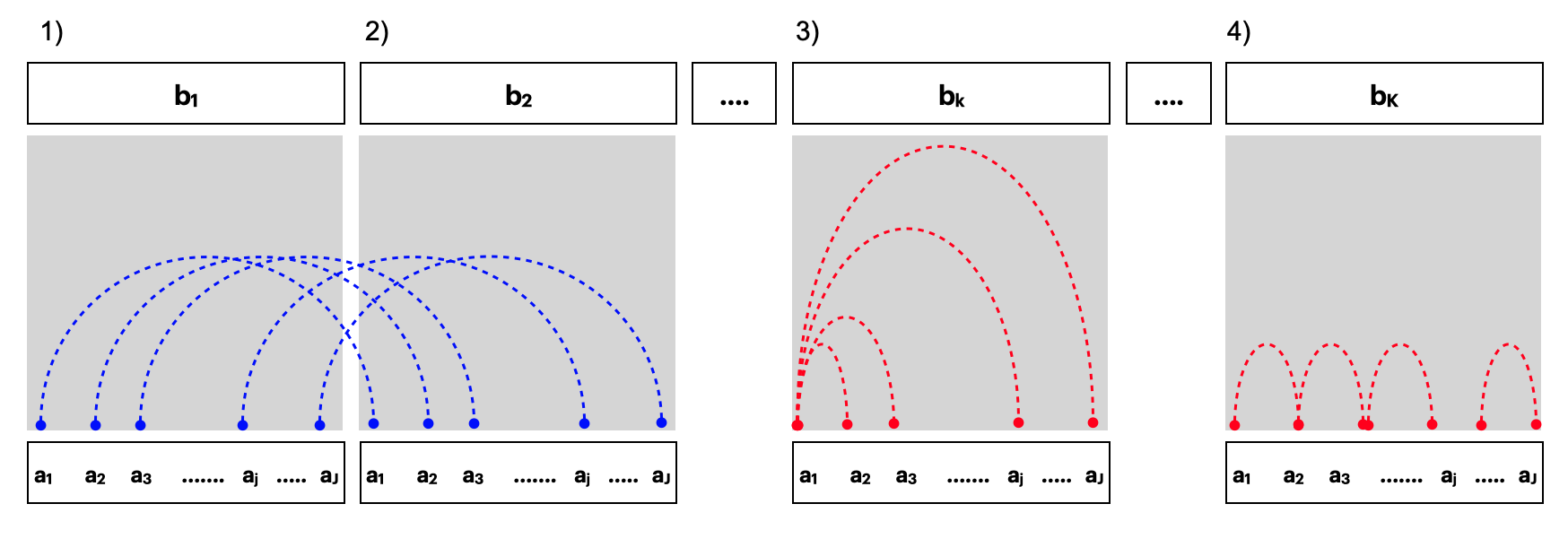
Figure 3.4: Within and between-facet distances shown for two cyclic granularities A and B, where A is mapped to x-axis and B is mapped to facets. The dotted lines represent the distances between different categories. Panels 1) and 2) show the between-facet distances. Panels 3) and 4) are used to illustrate within-facet distances when categories are un-ordered or ordered respectively. When categories are ordered, distances should only be considered for consecutive x-axis categories. Between-facet distances are distances between different facet levels for the same x-axis category; for example, distances between {(\(a_1\),\(b_1\)) and (\(a_1\), \(b_2\))} or {(\(a_1\),\(b_1\)) and (\(a_1\), \(b_3\))}.
Pairwise distances could be within-facets or between-facets for \(m = 2\). Figure illustrates how they are defined. Pairwise distances are within-facets when \(b_{k} = b_{k'}\), that is, between pairs of the form \((a_{j}b_{k}, a_{j'}b_{k})\) as shown in panel (3) of Figure . If categories are ordered (like all temporal cyclic granularities), then only distances between pairs where \(a_{j'} = (a_{j+1})\) are considered (panel (4)). Pairwise distances are between-facets when they are considered between pairs of the form \((a_{j}b_{k}, a_{j}b_{k'})\). There are a total of \({\nf \choose 2}\nx\) between-facet distances, and \({\nx \choose 2}\nf\) within-facet distances if they are ordered and \(\nf(\nx-1)\) within-facet distances if they are unordered.
Tuning parameter
For displays with \(m>1\) granularities, we can use a tuning parameter to specify the relative weight given to each granularity. In general, the tuning parameters should be chosen such that \(\sum_{i=1}^m \lambda_i = 1\).
Following the general principles of Gestalt theory, we wish to weight more heavily granularities that are plotted closer together. For \(m=2\) we choose \(\lambda_x = \frac{2}{3}\) for the granularity on the x-axis and \(\lambda_f = \frac13\) for the granularity mapped to facets, giving a relative weight of \(2:1\) for within-facet to between-facet distances. No human experiment has been conducted to justify this ratio. Specifying \(\lambda_x>0.5\) will weight within-facet distances more heavily, while \(\lambda_x <0.5\) would weight the between-facet distances more heavily. (See the supplements for more details.)
Raw distance measure
The raw distance measure, denoted by \(\wpdsub{raw}\), is computed after combining all the weighted distance measures appropriately. First, NQT is performed on the measured variable \(v_t\) to obtain \(v^*_t\) (data transformation). Then, for a fixed harmony pair \((A, B)\), percentiles of \(v^*_{jk}\) are computed and stored in \(q_{jk}\) (distribution characterization). This is repeated for all pairs of categories of the form \((a_{j} b_{k}, a_{j'}b_{k'}): \{a_j: j = 1, 2, \dots, \nx\}, B = \{ b_k: k = 1, 2, \dots, \nf\}\). The pairwise distances between pairs \((a_{j} b_{k}, a_{j'}b_{k'})\) denoted by \(d_{(jk, j'k')} = JSD(q_{jk}, q_{j'k'})\) are computed (distance between distributions). The pairwise distances (within-facet and between-facet) are transformed using a suitable tuning parameter (\(0<\lambda<1\)) depending on if they are within-facet(\(d_w\)) or between-facets(\(d_b\)) as follows: \[\begin{equation}\label{def:raw-wpd} d*_{(j,k), (j'k')} = \begin{cases} \lambda d_{(jk), (j'k')},& \text{if } d = d_w;\\ (1-\lambda) d_{(jk), (j'k')}, & \text{if } d = d_b. \end{cases} \end{equation}\] The \(\wpdsub{raw}\) is then computed as \[ \wpdsub{raw} = \max_{j, j', k, k'}(d*_{(jk), (j'k')}) \qquad\forall j, j' \in \{1, 2, \dots, \nx\},\quad k, k' \in \{1, 2, \dots, \nf\} \] The statistic “maximum” is chosen to combine the weighted pairwise distances since the distance measure is aimed at capturing the maximum variation of the measured variable within a panel. The statistic “maximum” is, however, affected by the number of comparisons (resulting pairwise distances). For example, for a \((2, 3)\) panel, there are \(6\) possible subsets of observations corresponding to the combinations \((a_1, b_1), (a_1, b_2), (a_1, b_3), (a_2 ,b_1), (a_2 ,b_2), (a_2, b_3)\), whereas for a \((2, 2)\) panel, there are only \(4\) possible subsets \((a_1, b_1), (a_1, b_2), (a_2 ,b_1), (a_2 ,b_2)\). Consequently, the measure would have higher values for the panel \((2, 3)\) as compared to \((2, 2)\), since maximum is taken over higher number of pairwise distances.
3.2.4 Adjusting for the number of comparisons
Ideally, it is desired that the proposed distance measure takes a higher value only if there is a significant difference between distributions across categories, and not because the number of categories \(\nx\) or \(\nf\) is high. That is, under designs like \(\Dnull\), their distribution should not differ for a different number of categories. Only then could the distance measure be compared across panels with different levels. This calls for an adjusted measure, which normalizes for the different number of comparisons.
Two approaches for adjusting the number of comparisons are discussed, both of which are substantiated using simulations. The first one defines an adjusted measure \(\wpdsub{perm}\) based on the permutation method to remove the effect of different comparisons. The second approach fits a model to represent the relationship between \(\wpdsub{raw}\) and the number of comparisons and defines the adjusted measure (\(\wpdsub{glm}\)) as the residual from the model.
Permutation approach
This method is somewhat similar in spirit to bootstrap or permutation tests, where the goal is to test the hypothesis that the groups under study have identical distributions. This method accomplishes a different goal of finding the null distribution for different groups (panels in our case) and standardizing the raw values using that distribution. The values of \(\wpdsub{raw}\) are computed on many (\(\nsub{perm}\)) permuted data sets and stored in \(\wpdsub{perm-data}\). Then \(\wpdsub{perm}\) is computed as follows: \[\begin{align*} \wpdsub{perm} = \frac{(\wpdsub{raw} - \text{mean}(\wpdsub{perm-data}))}{\text{sd}(\wpdsub{perm-data})} \end{align*}\] where \(\text{mean}(\wpdsub{perm-data})\) and \(\text{sd}(\wpdsub{perm-data})\) are the mean and standard deviation of \(\wpdsub{perm-data}\) respectively. Standardizing \(\wpd\) in the permutation approach ensures that the distribution of \(\wpdsub{perm}\) under \(\Dnull\) has zero mean and unit variance across all comparisons. While this works successfully to make the location and scale similar across different \(\nx\) and \(\nf\), it is computationally heavy and time consuming, and hence less user-friendly. Hence, another approach to adjustment, with potentially less computational time, is proposed.
Modeling approach
In this approach, a Gamma generalized linear model (GLM) for \(\wpdsub{raw}\) is fitted with the number of comparisons as the explanatory variable. Since, \(\wpdsub{raw}\) is a Jensen-Shannon distance, it follows a Chi-square distribution (Menéndez et al. 1997), which is a special case of a Gamma distribution. Furthermore, the mean response is bounded, since any JSD is bounded by \(1\) if a base \(2\) logarithm is used (Lin 1991). Hence, by Faraway (2016), an inverse link is used for the model, which is of the form \(y = a+b*\log(z) + e\), where \(y = \wpdsub{raw}\), \(z = (\nx*\nf)\) is the number of groups and \(e\) are idiosyncratic errors. Let \(\text{E}(y) = \mu\) and \(a + b*\log(z) = g(\mu)\) where \(g(\mu)= 1/\mu\) and \(\hat \mu = 1/(\hat a + \hat b \log(z))\). The residuals from this model \((y-\hat y) = (y-1/(\hat a + \hat b \log(z)))\) would be expected to have no dependency on \(z\). Thus, \(\wpdsub{glm}\) is defined as the residuals from this model given by \[\wpdsub{glm} = \wpdsub{raw} - 1/(\hat a + \hat b*\log(\nx*\nf))\] The distribution of \(\wpdsub{glm}\) under \(\Dnull\) will have approximately zero mean and a constant variance (not necessarily 1).
Combination approach
The simulation results (in Section ) show that the distribution of \(\wpdsub{glm}\) under the null design is similar for high \(\nx\) and \(\nf\) (levels higher than \(5\)) but less so for lower values of \(\nx\) and \(\nf\). Hence, a combination approach is proposed where we use a permutation approach for categories with small numbers of levels, and a modeling approach for categories with higher numbers of levels. This ensures that the computational load of the permutation approach is alleviated while maintaining a similar null distribution across different categories. This approach, however, requires that the adjusted variables from the two approaches are brought to the same scale. We define \(\wpdsub{glm-scaled} = \wpdsub{glm}*\sigma^2_{\text{perm}}/\sigma^2_{\text{glm}}\) as the transformed \(\wpdsub{glm}\) with a similar scale as \(\wpdsub{perm}\). The adjusted measure from the combination approach, denoted by \(\wpd\) is then defined as follows: \[\begin{equation} \wpd = \begin{cases} \wpdsub{perm}, & \text{if $\nx, \nf \le 5$};\\ \wpdsub{glm-scaled} & \text{otherwise}.\\ \end{cases} \end{equation}\]