4.2 Clustering methodology
The existing work on clustering probability distributions assumes we have an independent and identically distributed samples \(f_1(v),\dots,f_n(v)\), where \(f_i(v)\) denotes the distribution from observation \(i\) over some random variable \(v = \{v_t: t = 0, 1, 2, \dots, T-1\}\) observed across \(T\) time points. In our approach, instead of considering the probability distributions of the linear time series, we compare them across different categories of a cyclic granularity. We can consider categories of an individual cyclic granularity (\(A\)) or combination of categories for two interacting granularities (\(A*B\)) to have a distribution, where \(A, B\) are defined as \(A = \{a_j: j=1, 2, \dots J\}\) and \(B = \{b_k: k = 1, 2, \dots K\}\). For example, let us consider two cyclic granularities, \(A\) and \(B\), representing hour-of-day and day-of-week, repsectively. Then \(A = \{0, 1, 2, \dots, 23\}\) and \(B = \{Mon, Tue, Wed, \dots, Sun\}\). In case individual granularities are considered, there are \(J = 24\) distributions of the form \(f_{i,j}(v)\) or \(K = 7\) distributions of the form \(f_{i,k}(v)\) for each customer \(i\). In case of interaction, \(J*K=168\) distributions of the form \(f_{i,j, k}(v)\) could be conceived for each customer \(i\). Hence clustering these customers is equivalent to clustering these collections of conditional univariate probability distributions. Towards this goal, the next step is to decide how to measure distances between collections of univariate probability distributions. Here, we describe two approaches for finding distances between time series. Both of these approaches may be useful in a practical context, and produce very different but equally useful customer groupings. The distances can be supplied to any usual clustering algorithm, including \(k\)-means or hierarchical clustering, to group observations into a smaller more homogeneous collection. The flow of the procedures is illustrated in Figure .
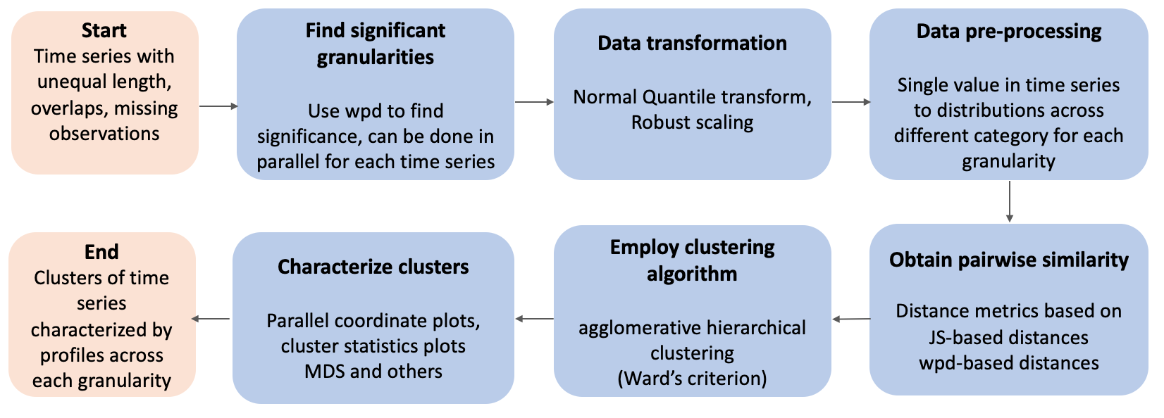
Figure 4.1: Flow chart illustrating the pipeline for out method for clustering time series.
4.2.1 Selecting granularities
(Gupta, Hyndman, and Cook 2021) provides a method for determining the significance of a cyclic granularity, and a ranking of multiple cyclic granularities. (This extends to harmonies, pairs of granularities that might interact with each other.) We define “significant” granularities as those with significant distributional differences across at least one category. The reason for subsetting granularities in this way, is that, clustering algorithms perform badly in the presence of nuisance variables. Granularities that do not have some difference between categories are likely to be nuisance variables. It should be noted that all of the time series in a collection may not have the same set of significant granularities. This is the approach for managing this generate a subset (\(S_c\)) of significant granularities across a collection of time series:
Remove granularities from the comprehensive list that are not significant for any time series.
Select only the granularities that are significant for the majority of time series.
4.2.2 Data transformation
The shape and scale of the distribution of the measured variable (e.g. energy usage) affects distance calculations. Skewed distributions need to be symmetrized. Scales of individuals needs to be standardized, because clustering is to select similar patterns, not magnitude of usage. (Organizing individuals based on magnitude can achieved simply by sorting on a statistic like the average value across time.) For the JS-based approaches, two data transformation techniques are recommended, normal-quantile transform (NQT) and robust scaling (RS). NQT is used in @Gupta, Hyndman, and Cook (2021) prior sorting granularities.
RS: The normalized \(i^{th}\) observation is denoted by \(v_{norm} = \frac{v_t - q_{0.5}}{q_{0.75}-q_{0.25}}\), where \(v_t\) is the actual value at the \(t^{th}\) time point and \(q_{0.25}\), \(q_{0.5}\) and \(q_{0.75}\) are the \(25^{th}\), \(50^{th}\) and \(75^{th}\) percentile of the time series for the \(i^{th}\) observation. Note that, \(v_{norm}\) has zero mean and median, but otherwise the shape does not change.
NQT: The raw data for all observations is individually transformed (Krzysztofowicz 1997), so that the transformed data follows a standard normal distribution. NQT will symmetrize skewed distributions. A drawback is that any multimodality will be concealed. This, this should be checked prior to applying NQT.
4.2.3 Data pre-preprocessing
Computationally in R, the data is assumed to be a “tsibble object” (Wang, Cook, and Hyndman (2020a)) equipped with an index variable representing inherent ordering from past to present and a key variable that defines observational units over time. The measured variable for an observation is a time-indexed sequence of values. This sequence, however, could be shown in several ways. A shuffle of the raw sequence may represent hourly consumption throughout a day, a week, or a year. Cyclic granularities can be expressed in terms of the index set in the tsibble data structure.
The data object will change when cyclic granularities are computed, as multiple observations will be categorized into levels of the granularity, thus inducing multiple probability distributions. Directly computing Jensen-Shannon distances between the entire probability distributions can be computationally intensive. Thus it is recommended that quantiles are used to characterize the probability distributions. In the final data object, each category of a cyclic granularity corresponds to a list of numbers which is composed of a few quantiles.
4.2.4 Distance metrics
The total (dis) similarity between each pair of customers is obtained by combining the distances between the collections of conditional distributions. This needs to be done in a way such that the resulting metric is a distance metric, and could be fed into the clustering algorithm. Two types of distance metrics are considered:
4.2.4.1 JS-based distances
This distance metric considers two time series to be similar if the distributions of each category of an individual cyclic granularity or combination of categories for interacting cyclic granularities are similar. In this study, the distribution for each category is characterized using deciles (can potentially consider any list of quantiles), and the distances between distributions are calculated using the Jensen-Shannon distances (Menéndez et al. (1997)), which are symmetric and thus could be used as a distance measure.
The sum of the distances between two observations \(x\) and \(y\) in terms of cyclic granularity \(A\) is defined as \[S^A_{x,y} = \sum_{j} D_{x,y}(A)\] (sum of distances between each category \(j\) of cyclic granularity \(A\)) or \[S^{A*B}_{x,y} = \sum_j \sum_k D_{x,y}(A, B)\] (sum of distances between each combination of categories \((j, k)\) of the harmony \((A, B)\)). After determining the distance between two series in terms of one granularity, we must combine them to produce a distance based on all significant granularities. When combining distances from individual \(L\) cyclic granularities \(C_l\) with \(n_l\) levels, \[S_{x, y} = \sum_lS^{C_l}_{x,y}/n_l\] is employed, which is also a distance metric since it is the sum of JS distances. This approach is expected to yield groups, such that the variation in observations within each group is in magnitude rather than distributional pattern, while the variation between groups is only in distributional pattern across categories.
4.2.4.2 wpd-based distances
Compute weighted pairwise distances \(wpd\) (Gupta, Hyndman, and Cook (2021)) for all considered granularities for all observations. \(wpd\) is designed to capture the maximum variation in the measured variable explained by an individual cyclic granularity or their interaction and is estimated by the maximum pairwise distances between consecutive categories normalized by appropriate parameters. A higher value of \(wpd\) indicates that some interesting patterns are expected, whereas a lower value would indicate otherwise.
Once we have chosen \(wpd\) as a relevant feature for characterizing the distributions across one cyclic granularity, we have to decide how we combine differences between the multiple features (corresponding to multiple granularities) into a single number. The Euclidean distance between them is chosen, with the granularities acting as variables and \(wpd\) representing the value under each variable. With this approach, we should expect the observations with similar \(wpd\) values to be clustered together. Thus, this approach is useful for grouping observations that have a similar significance of patterns across different granularities. Similar significance does not imply a similar pattern, which is where this technique varies from JS-based distances, which detect differences in patterns across categories.
4.2.5 Clustering
4.2.5.1 Number of clusters
Different approaches to determining number of clusters are required for varied applications and research objectives. It is often beneficial to investigate numerous cluster statistics in order to arrive at a number of clusters, since clustering has a variety of objectives (e.g., between-cluster separation, within-cluster homogeneity, representation by centroids, etc.), which could be in conflict with one another. Some typical ways of determining the number of clusters in the literature (e.g., the gap statistic (Tibshirani, Walther, and Hastie 2001), average silhouette width (Rousseeuw 1987), Dunn index (Dunn 1973)) are inspired by defining and balancing “within-cluster homogeneity” and “between-cluster separation.” The Cluster separation index (\(sindex\)) proposed by Hennig (2014) is used as a guide to select the number of clusters in Section . \(sindex\) (Hennig 2020) is a compromise between minimum cluster separation and average cluster separation and is less sensitive to a single or few ambiguous points. \(sindex\) cannot be optimized over the number of clusters, since increasing the number of clusters reduces it. The number of clusters required is determined by the slope going from steep to shallow (an elbow).
.
4.2.5.2 Algorithm
With a way to obtain pairwise distances, any clustering algorithm can be employed that supports the given distance metric as input. A good comprehensive list of algorithms can be found in Xu and Tian (2015) based on traditional ways like partition, hierarchy, or more recent approaches like distribution, density, and others. We employ agglomerative hierarchical clustering in conjunction with Ward’s linkage. Hierarchical cluster techniques fuse neighboring points sequentially to form bigger clusters, beginning with a full pairwise distance matrix. The distance between clusters is described using a “linkage technique.” This agglomerative approach successively merges the pair of clusters with the shortest between-cluster distance using Ward’s linkage method.
4.2.5.3 Characterization of clusters
Cluster characterization is an important element of cluster analysis. Cook and Swayne (2007) provides several methods for characterizing clusters. Parallel coordinate plots (Wegman (1990)), Scatterplot matrix, Displaying cluster statistics (Dasu, Swayne, and Poole (2005)), MDS (Borg and Groenen (2005)), PCA, t-SNE(Krijthe (2015)), Tour (Wickham et al. (2011)) are some of the graphical approaches used in this study. A Parallel Coordinates Plot features parallel axes for each variable and each axis is linked by lines. Changing the axes may reveal patterns or relationships between variables for categorical variables. However, for categories with cyclic temporal granularities, preserving the underlying ordering of time is more desirable. Displaying cluster statistics is useful when we have larger problems and it is difficult to read the parallel coordinate plots due to congestion. All of MDS, PCA and t-SNE use a distance or dissimilarity matrix to construct a reduced-dimension space representation, but their goals are diverse. Multidimensional scaling (Borg and Groenen (2005)) seeks to maintain the distances between pairs of data points, with an emphasis on pairings of distant points in the original space. The t-SNE embedding will compress data points that are close in high-dimensional space. Tour is a collection of interpolated linear projections of multivariate data into lower-dimensional space. The cluster characterization approach varies depending on the distance metric used. Parallel coordinate plots, scatter plot matrices, MDS or PCA are potentially useful ways to characterize clusters using wpd-based distances. For JS-based distances, plotting cluster statistics is beneficial for characterization and variable importance could be displayed through parallel coordinate plots.