4.3 Validation

To validate our clustering methods, we spiked many attributes in the data to create different data designs. Three circular granularities $g1$, $g2$ and $g3$ are considered with categories denoted by $\{g10,g11\}$, $\{g20, g21, g22\}$ and $\{g30, g31, g32, g33, g34\}$ and levels $n_{g_1}=2$, $n_{g_2}=3$ and $n_{g_3}=5$. These categories could be integers or some more meaningful labels. For example, the granularity “day-of-week” could be either represented by $\{0, 1, 2, \dots, 6\}$ or $\{Mon, Tue, \dots, Sun\}$. Here categories of $g1$, $g2$ and $g3$ are represented by $\{0, 1\}$, $\{0, 1, 2\}$ and $\{0, 1, 2, 3, 4\}$ respectively. A continuous measured variable $v$ of length $T$ indexed by $\{0, 1, \dots T-1\}$ is simulated such that it follows the structure across $g1$, $g2$ and $g3$. We constructed independent replications of all data designs $R = \{25, 250, 500\}$ to investigate if our proposed clustering method can discover distinct designs in small, medium, and big numbers of series. All designs employ $T=\{300, 1000, 5000\}$ sample sizes to evaluate small, medium, and large-sized series. Variations in method performance may be due to different jumps between categories. So a mean difference of $\mu = \{1, 2, 5\}$ between categories is considered. The performance of the approaches varies with the number of granularities which has interesting patterns across its categories. So three scenarios are considered to accommodate that. Figure shows the range of parameters considered for each scenario.

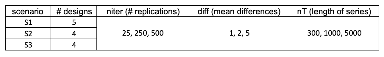
Figure 4.2: Range of parameters for different scenarios

4.3.1 Data generation

Each category or combination of categories from $g1$, $g2$ and $g3$ are assumed to come from the same distribution, a subset of them from the same distribution, a subset of them from separate distributions, or all from different distributions, resulting in various data designs. As the methods ignore the linear progression of time, there is little value in adding time dependency to the data generating process. The data type is set to be “continuous,” and the setup is assumed to be Gaussian. When the distribution of a granularity is “fixed,” it means distributions across categories do not vary and are considered to be from N (0,1). $\mu$ alters in the “varying” designs, leading to varying distributions across categories.

4.3.2 Data designs

4.3.2.1 Individual granularities

Scenario (S1): All granularities significant

Consider the instance where $g1$, $g2$, and $g3$ all contribute to design distinction. This means that each granularity will have significantly different patterns at least across one of the designs to be clustered. In Table various distributions across categories are considered (top) which lead to different designs (bottom). Figure shows the simulated variable’s linear (left) and cyclic (right) representations for each of these five designs. The structural difference in the time series variable is impossible to discern from the linear view, with all of them looking very similar. The shift in structure may be seen clearly in the distribution of cyclic granularities. The following scenarios use solely graphical displays across cyclic granularities to highlight distributional differences in categories.

Scenario (S2): Few significant granularities

This is the case where one granularity will remain the same across all designs. We consider the case where the distribution of $v$ varies across $g2$ levels for all designs, across $g3$ levels for a few designs, and $g1$ does not vary across designs. The proposed design is shown in Figure (b).

Scenario (S3): Only one significant granularity

Only one granularity is responsible for identifying the designs in this case. This is depicted in Figure (right) where only $g3$ affects the designs significantly.

Table 4.1: For S1, distributions of different categories when they vary (displayed on top). If distributions are fixed, they are set to N(0, 1). The various distributions across categories result in five designs (displayed below).

granularity	Varying distributions
g1	g10 ~ N(0, 1), g11 ~ N(2, 1)
g2	g21 ~ N(2, 1), g22 ~ N(1, 1), g23 ~ N(0, 1)
g3	g31 ~ N(0, 1), g32 ~ N(1, 1), g33 ~ N(2, 1), g34 ~ N(1, 1), g35 ~ N(0, 1)

design	g1	g2	g3
design-1	fixed	fixed	fixed
design-2	vary	fixed	fixed
design-3	fixed	vary	fixed
design-4	fixed	fixed	vary
design-5	vary	vary	vary

The linear (left) and cyclic (right) representation is shown under scenario S1 using line plots and boxplots respectively. Each row represents a design. Distributions of categories across $g1$, $g2$ and $g3$ change across at least one design as can be observed in the cyclic representation. It is not possible to comprehend these structural differences in patterns just by looking at or considering the linear representation.

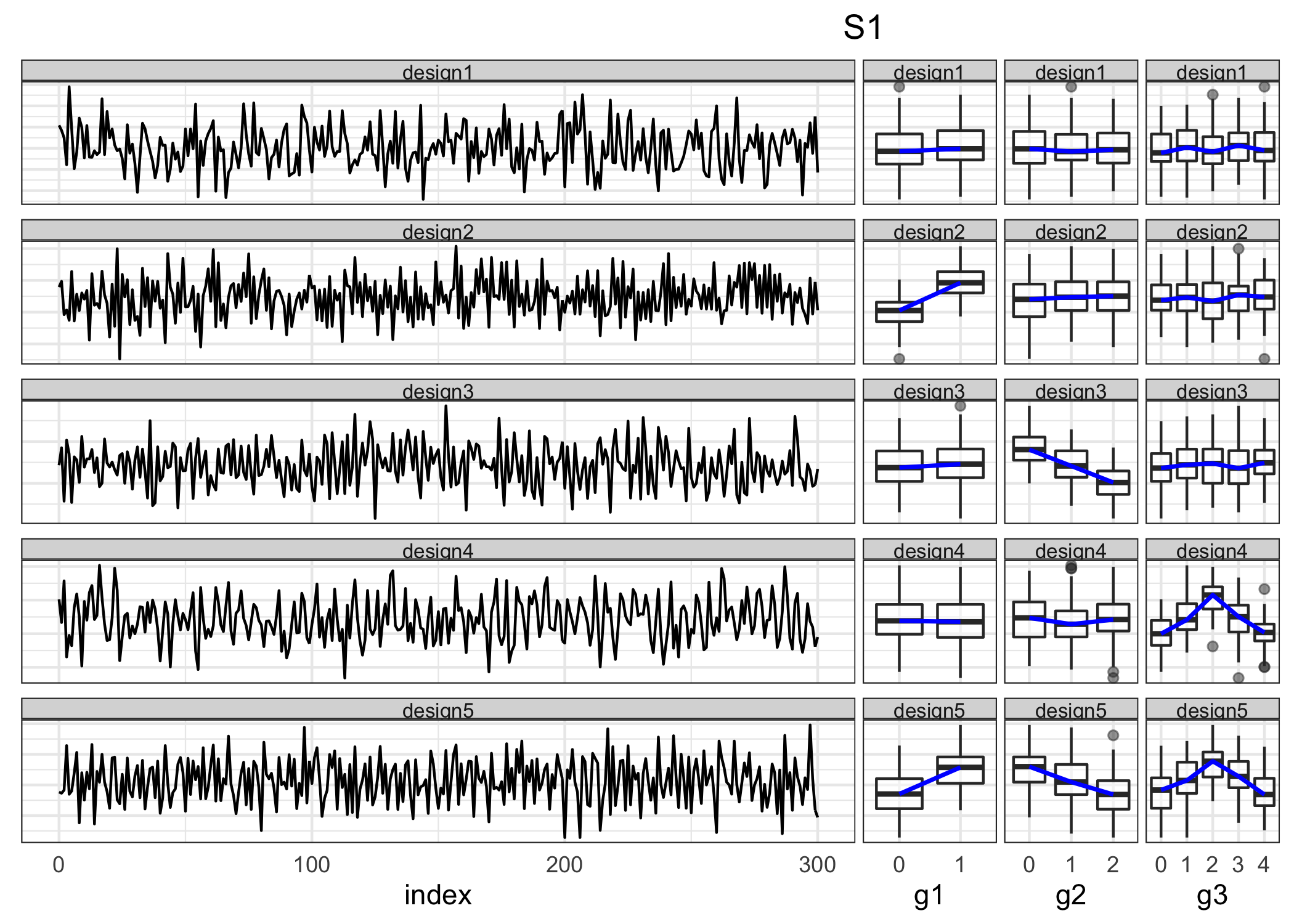
Figure 4.3: The linear (left) and cyclic (right) representation is shown under scenario S1 using line plots and boxplots respectively. Each row represents a design. Distributions of categories across $g1$, $g2$ and $g3$ change across at least one design as can be observed in the cyclic representation. It is not possible to comprehend these structural differences in patterns just by looking at or considering the linear representation.

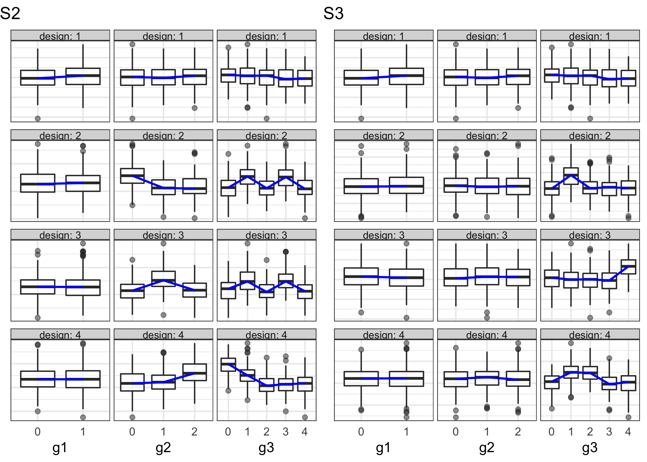
Boxplots showing distributions of categories across different designs (rows) and granularities (columns) for scenarios S2 and S3. In S2, $g2$, $g3$ change across at least one design but $g1$ remains constant. Only $g3$ changes across different designs in S3.

Figure 4.4: Boxplots showing distributions of categories across different designs (rows) and granularities (columns) for scenarios S2 and S3. In S2, $g2$, $g3$ change across at least one design but $g1$ remains constant. Only $g3$ changes across different designs in S3.

4.3.2.2 Interaction of granularities

The proposed methods could be extended when two granularities of interest interact and we want to group subjects based on the interaction of the two granularities. Consider a group that has a different weekday and weekend behavior in the summer but not in the winter. This type of combined behavior across granularities can be discovered by evaluating the distribution across combinations of categories for different interacting granularities (weekend/weekday and month-of-year in this example). As a result, in this scenario, we analyze a combination of categories generated from different distributions. Display of design and related results can be found in supplementary.

4.3.3 Visual exploration of results

All of the approaches were fitted to each data design and to each combination of the considered parameters. The formed clusters have to match the design, be well separated, and have minimal intra-cluster variation. It is possible to study these desired clustering traits visually in a more comprehensive way than just looking at index values. MDS and parallel coordinate graphs are used to demonstrate the findings, as well as an index value plot to provide direction on the number of clusters. JS-based approaches corresponding to NQT and RS are referred to as JS-NQT and JS-RS respectively. In the following plots, results for JS-NQT are reported. For similar results with JS-RS or wpd-based distances, please refer to the supplementary paper.

Figure shows $sindex$ plotted against the number of clusters ($k$) for the range of mean differences (rows) under the different scenarios (columns). This can be used to determine the number of clusters for each scenario. When $sindex$ for each scenario are examined, it appears that $k = 5, 4, 4$ is justified for scenarios S1, S2, and S3, respectively, given the sharp decrease in $sindex$ from that value of $k$. Thus, the number of clusters corresponds to the number of designs that were originally considered in each scenario.
Figure shows separation of our clusters. It can be observed that in all scenarios and for different mean differences, clusters are separated. However, the separation increases with an increase in mean differences across scenarios. This is intuitive because, as the difference between categories increases, it gets easier for the methods to correctly distinguish the designs.
Figure depicts a parallel coordinate plot with the vertical bar showing total inter-cluster distances with regard to granularities $g1$, $g2$, and $g3$ for all simulation settings and scenarios. So one line in the figure shows the inter-cluster distances for one simulation setting and scenarios vary across facets. The lines are not colored by group since the purpose is to highlight the contribution of the factors to categorization rather than class separation. Panel S1 shows that no variable stands out in the clustering, but the following two panels show that {g1} and {g1, g2} have very low inter-cluster distances, meaning that they did not contribute to the clustering. It is worth noting that these facts correspond to our original assumptions when developing the scenarios, which incorporate distributional differences over three (S1), two (S2), and one (S3) significant granularities. Hence, Figure (S1), (S2), and (S3) validate the construction of scenarios (S1), (S2), and (S3) respectively.
The JS-RS and wpd-based methods perform worse for $nT=300$, then improve for higher $nT$ evaluated in the study. However, a complete year of data is the minimum requirement to capture distributional differences in winter and summer profiles, for example. Even if the data is only available for a month, $nT$ with half-hourly data is expected to be at least $1000$. As a result, as long as the performance is promising for higher $nT$, this is not a challenge.
In our study sample, the method JS-NQT outperforms the method JS-RS for smaller differences between categories. More testing, however, is required to corroborate this.

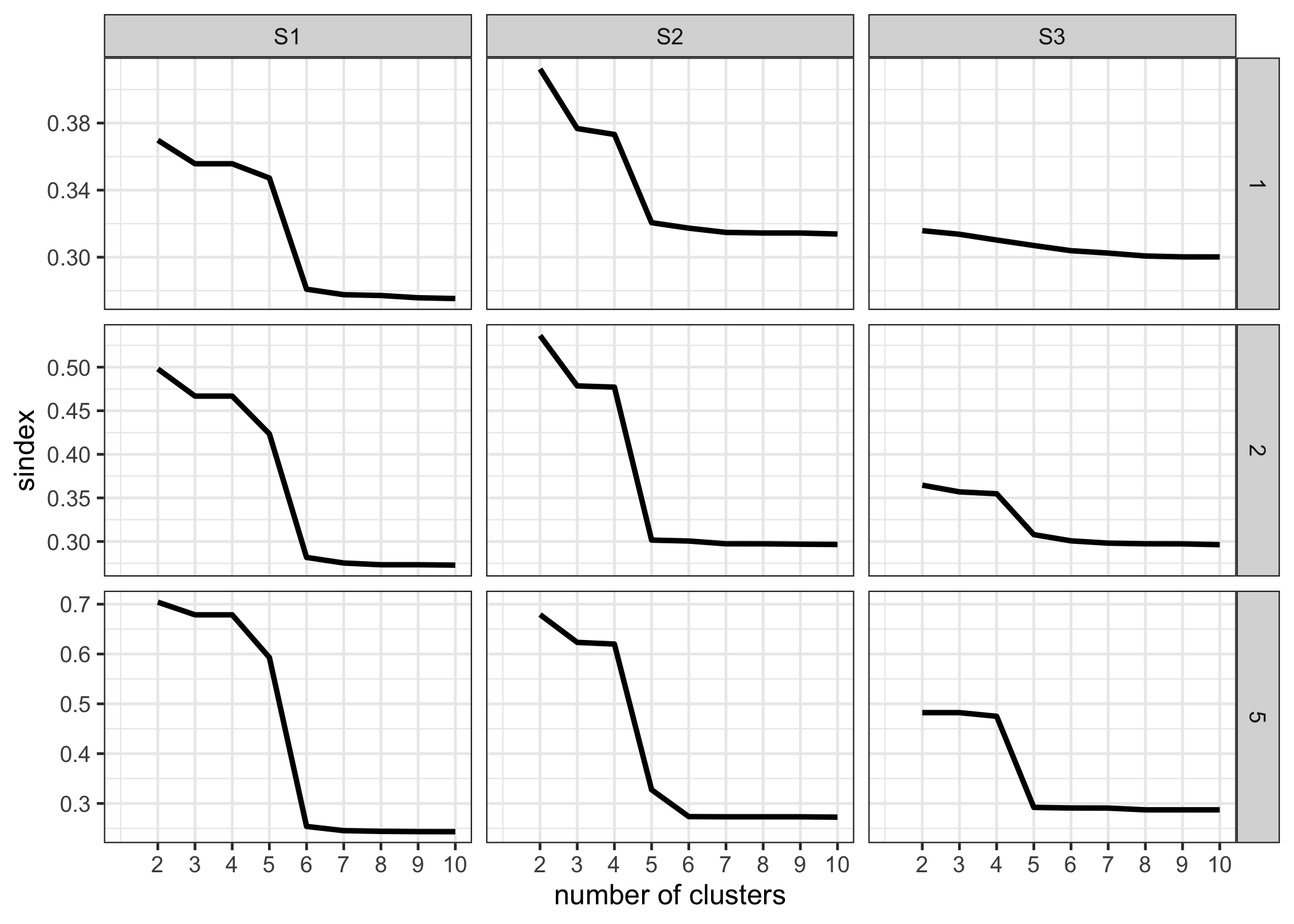
The cluster separation index (sindex) is plotted as a function of the number of clusters for the range of mean differences (rows) under the different scenarios (columns). S1 has a sharp decrease in sindex from 5 to 6, whereas S2 and S3 have a decrease from 4 to 5. As a result, the number of clusters considered for S1, S2, and S3 is 5, 4, 4, respectively. This corresponds to the number of designs taken into account in each scenario.

Figure 4.5: The cluster separation index (sindex) is plotted as a function of the number of clusters for the range of mean differences (rows) under the different scenarios (columns). S1 has a sharp decrease in sindex from 5 to 6, whereas S2 and S3 have a decrease from 4 to 5. As a result, the number of clusters considered for S1, S2, and S3 is 5, 4, 4, respectively. This corresponds to the number of designs taken into account in each scenario.

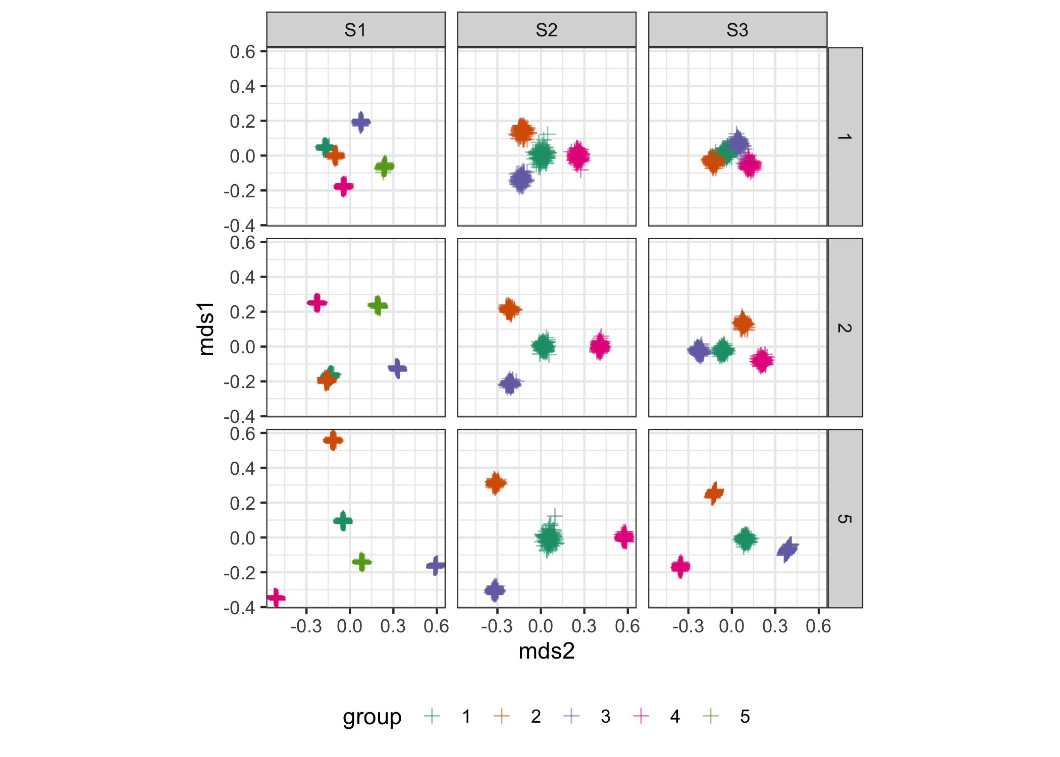
MDS summary plots to illustrate the cluster sparation for the range of mean differences (rows) under the different scenarios (columns). It can be observed that clusters become more compact and separated for higher mean differences between categories across all scenarios. Between scenarios, separation is least prominent corresponding to Scenario (S3) where only one granularity is responsible for distinguishing the clusters.

Figure 4.6: MDS summary plots to illustrate the cluster sparation for the range of mean differences (rows) under the different scenarios (columns). It can be observed that clusters become more compact and separated for higher mean differences between categories across all scenarios. Between scenarios, separation is least prominent corresponding to Scenario (S3) where only one granularity is responsible for distinguishing the clusters.

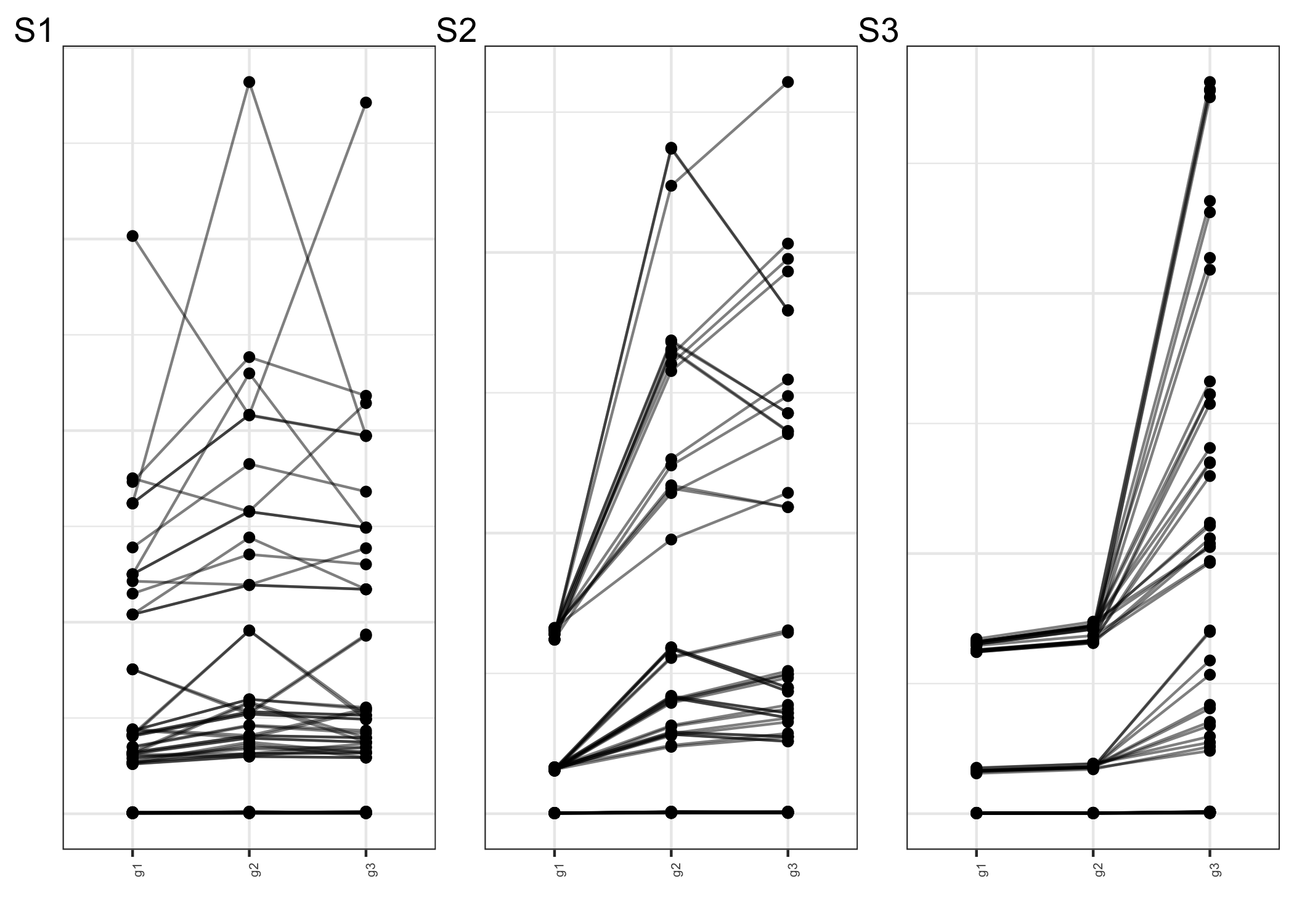
The parallel coordinate figure depicts total inter-cluster distances for the granularities $g1$, $g2$, and $g3$. The inter-cluster distances for a single simulation scenario are represented by one line in the figure. While panel S1 shows that no variable stands out during clustering, panels S2 and S3 show that g1 and (g1, g2) had smaller inter-cluster distances, indicating that they did not contribute to clustering. These facts are consistent with our initial assumptions when building the scenarios, and S1, S2, S3 correspond to scenarios with three, two, and one significant granularity, respectively.

Figure 4.7: The parallel coordinate figure depicts total inter-cluster distances for the granularities $g1$, $g2$, and $g3$. The inter-cluster distances for a single simulation scenario are represented by one line in the figure. While panel S1 shows that no variable stands out during clustering, panels S2 and S3 show that g1 and (g1, g2) had smaller inter-cluster distances, indicating that they did not contribute to clustering. These facts are consistent with our initial assumptions when building the scenarios, and S1, S2, S3 correspond to scenarios with three, two, and one significant granularity, respectively.