Exploring probability distributions for cricket
Sayani Gupta
Source: vignettes/cricket.Rmd
cricket.RmdIntroduction
Package gravitas is not only restricted to temporal data. An application on cricket follows to illustrate how this package can be generalized in other applications.
The Indian Premier League (IPL) is a professional Twenty20 cricket league in India contested by teams representing different cities in India. In a Twenty20 game, the two teams have a single innings each, which is restricted to a maximum of 20 overs. Hence, in this format of cricket, a match will consist of 2 innings, an innings will consist of 20 overs, an over will consist of 6 balls. Therefore, a hierarchy can be construed for this game format.
The ball by ball data for IPL season is sourced from Kaggle. The cricket data set in the gravitas package summarizes the ball-by-ball data cross overs and contains information for a sample of 214 matches spanning 9 seasons (2008 to 2016).
library(gravitas)
library(tibble)
glimpse(cricket)
#> Rows: 8,560
#> Columns: 10
#> $ season        <dbl> 2008, 2008, 2008, 2008, 2008, 2008, 2008, 2008, 2008, 2…
#> $ match_id      <dbl> 2, 2, 2, 2, 2, 2, 2, 2, 2, 2, 2, 2, 2, 2, 2, 2, 2, 2, 2…
#> $ batting_team  <chr> "Chennai Super Kings", "Chennai Super Kings", "Chennai …
#> $ bowling_team  <chr> "Kings XI Punjab", "Kings XI Punjab", "Kings XI Punjab"…
#> $ inning        <dbl> 1, 1, 1, 1, 1, 1, 1, 1, 1, 1, 1, 1, 1, 1, 1, 1, 1, 1, 1…
#> $ over          <dbl> 1, 2, 3, 4, 5, 6, 7, 8, 9, 10, 11, 12, 13, 14, 15, 16, …
#> $ wicket        <dbl> 0, 0, 1, 0, 0, 0, 1, 1, 0, 0, 0, 0, 1, 0, 0, 1, 0, 0, 0…
#> $ dot_balls     <dbl> 4, 2, 4, 3, 3, 3, 1, 3, 1, 2, 1, 0, 2, 1, 0, 3, 0, 1, 0…
#> $ runs_per_over <dbl> 5, 14, 2, 6, 9, 11, 9, 8, 13, 5, 19, 20, 4, 10, 18, 8, …
#> $ run_rate      <dbl> 1, 2, 0, 1, 2, 2, 2, 1, 2, 1, 3, 3, 1, 2, 3, 1, 2, 3, 2…
Although there is no conventional time granularity in cricket, we can still represent the data set cricket through a tsibble, where each over, which represents an ordering from past to future, can form the index of the tsibble. The hierarchy table would look like the following:
hierarchy_model <- tibble::tibble(
  units = c("index", "over", "inning", "match"),
  convert_fct = c(1, 20, 2, 1))

knitr::kable(hierarchy_model, format = "markdown")
| units | convert_fct |
|---|---|
| index | 1 |
| over | 20 |
| inning | 2 |
| match | 1 |
library(tsibble)
cricket_tsibble <- cricket %>%
  mutate(data_index = row_number()) %>%
  as_tsibble(index = data_index)
How run rates vary depending on if a team bats first or second?
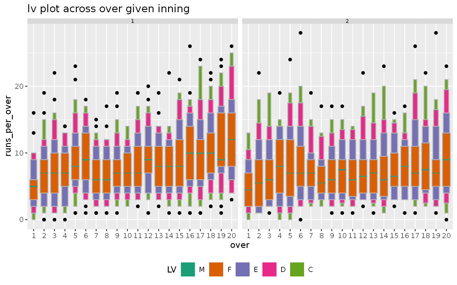
We filtered the data for two top teams in IPL - Mumbai Indians and Chennai Super Kings. Each inning of the match is plotted across facets and overs of the innings are plotted across the x-axis. It can be observed from the letter value plot that there is no clear upward shift in runs in the second innings as compared to the first innings. The variability of runs increases as the teams approach towards the end of the innings, as observed through the longer and more distinct letter values.
cricket_tsibble %>%
  filter(batting_team %in% c("Mumbai Indians",
                             "Chennai Super Kings"))%>%
  prob_plot("inning", "over",
  hierarchy_model,
  response = "runs_per_over",
  plot_type = "lv")
#> Joining, by = c("inning", "over")
#> Joining, by = c("inning", "over")

Do wickets and dot balls affect the runs differently across overs?
A dot ball is a delivery bowled without any runs scored off it. The number of dot balls is reflective of the quality of bowling in the game. The number of wickets per over can be thought to be a measure of good fielding. It might be interesting to see how good fielding or bowling effect runs per over differently.
Now, the number of wickets/dot balls per over does not appear in the hierarchy table, but they can still be thought of as granularities since they are constructed for each index (over) of the tsibble. The relationship is not periodic because of the number of wickets that are dismissed or dot balls that are being bowled changes across overs. This is unlike the periodic relationship for units specified in the hierarchy table.
gran_advice is employed to check if it would be appropriate to plot wickets and dot balls across overs. The output suggests that the pairs (dot_balls, over) and (wicket, over) are clashes. It also gives us the number of observations per categorization. The number of observations of 2, 3 or 4 wickets are too few to plot a distribution, implying there are hardly any overs in which 2 or more wickets are dismissed. The number of observations for more than 5 dot balls in any over is again very low suggesting those are even rarer cases.
cricket_tsibble %>%
  gran_advice("wicket",
            "over",
            hierarchy_model)
#> The chosen granularities are clashes.
#>         Consider looking at harmony() to obtain possible harmonies
#>
#> Recommended plots are: violin lv quantile boxplot
#>
#> Number of observations are homogenous across facets
#>
#> Number of observations are homogenous within facets
#>
#> Cross tabulation of granularities :
#>
#> # A tibble: 20 x 6
#>    over    `0`   `1`   `2`   `3`   `4`
#>    <fct> <dbl> <dbl> <dbl> <dbl> <dbl>
#>  1 1       355    67     6     0     0
#>  2 2       335    85     8     0     0
#>  3 3       335    85     8     0     0
#>  4 4       330    93     5     0     0
#>  5 5       328    95     5     0     0
#>  6 6       329    95     4     0     0
#>  7 7       346    79     3     0     0
#>  8 8       353    68     7     0     0
#>  9 9       323    99     6     0     0
#> 10 10      341    81     6     0     0
#> 11 11      320    97    11     0     0
#> 12 12      319   101     8     0     0
#> 13 13      322   100     6     0     0
#> 14 14      325    92    11     0     0
#> 15 15      291   126     9     2     0
#> 16 16      294   124    10     0     0
#> 17 17      268   141    17     2     0
#> 18 18      251   140    35     2     0
#> 19 19      242   140    43     3     0
#> 20 20      182   169    67     9     1
cricket_tsibble %>%
  gran_advice("dot_balls",
            "over",
            hierarchy_model)
#> The chosen granularities are clashes.
#>         Consider looking at harmony() to obtain possible harmonies
#>
#> Recommended plots are: quantile
#>
#> Number of observations are homogenous across facets
#>
#> Number of observations are homogenous within facets
#>
#> Cross tabulation of granularities :
#>
#> # A tibble: 20 x 8
#>    over    `0`   `1`   `2`   `3`   `4`   `5`   `6`
#>    <fct> <dbl> <dbl> <dbl> <dbl> <dbl> <dbl> <dbl>
#>  1 1         2    18    74   126   125    68    15
#>  2 2         6    38    80   133   105    57     9
#>  3 3        14    41   113   135    90    31     4
#>  4 4        17    62   114   124    80    25     6
#>  5 5        21    70   104   110    86    34     3
#>  6 6        20    66   111   125    76    24     6
#>  7 7        41   105   123   104    44    11     0
#>  8 8        53   105   129    82    44    15     0
#>  9 9        45   122   125    78    44    12     2
#> 10 10       52   141   109    83    35     7     1
#> 11 11       61   112   125    86    36     7     1
#> 12 12       69   137   117    71    27     7     0
#> 13 13       70   116   114    89    33     5     1
#> 14 14       62   134   114    81    22    14     1
#> 15 15       63   125   133    73    30     4     0
#> 16 16       80   148   121    49    20     9     1
#> 17 17       81   148   107    58    25     9     0
#> 18 18       72   128   145    57    24     2     0
#> 19 19       77   146   108    66    25     6     0
#> 20 20       72   141   117    62    29     6     1
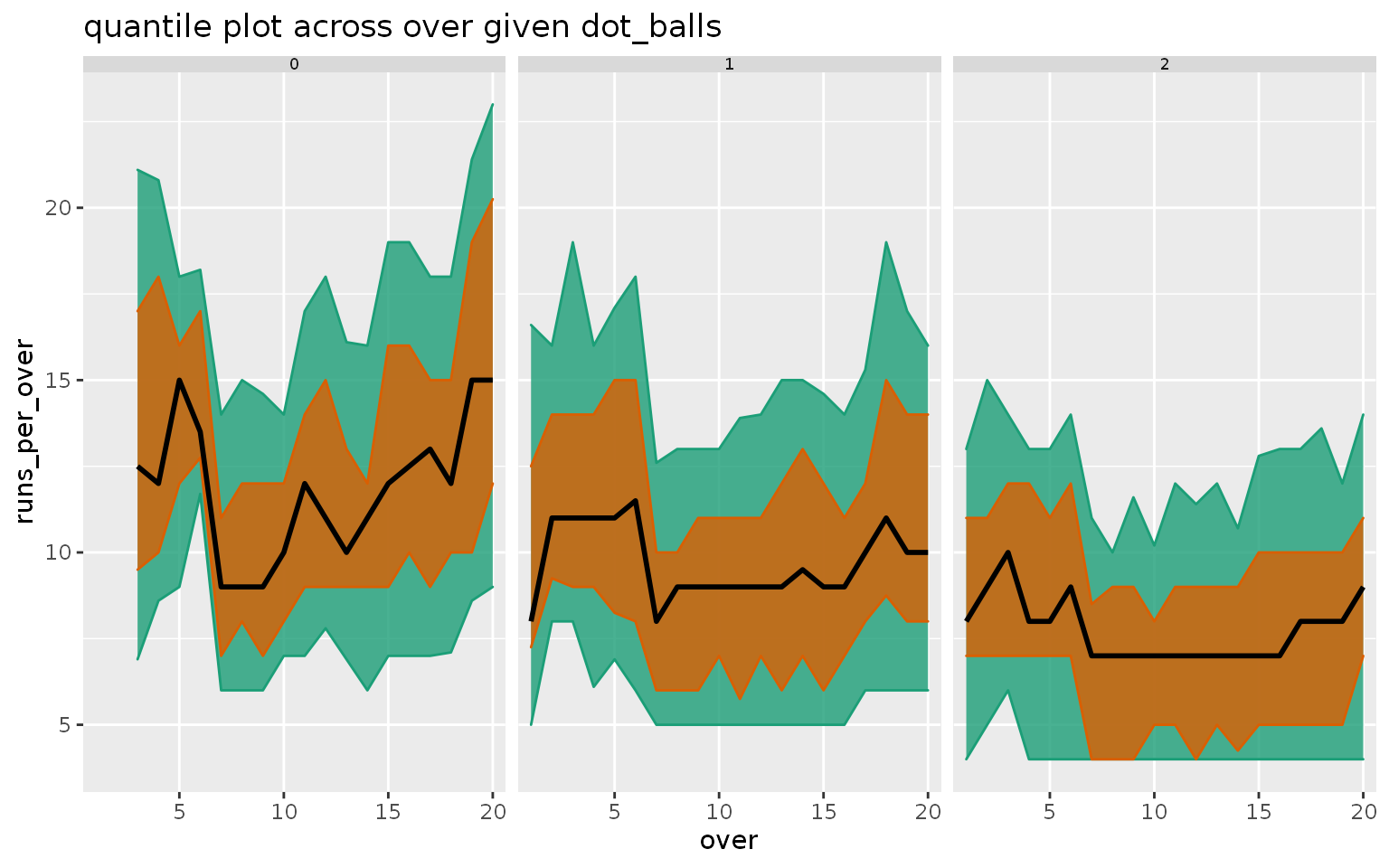
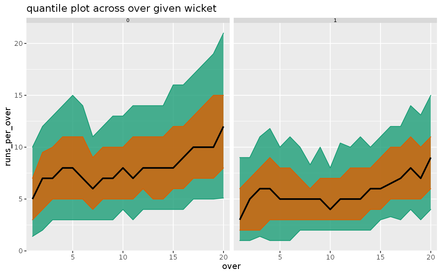
Hence, we filter our data set to retain those overs where the number of wickets or dot balls are less than, or equal to 2. Some pairs of granularities should still be analyzed with caution as suggested by gran_advice. Area quantile plots are drawn across overs of the innings, faceted by either number of dot balls (first) or the number of wickets (second). The dark black line represents the median, whereas the orange and green represent the area between the 25th and 75th percentile and between the 10th and 90th percentile respectively. For both the plots, runs per over decreases as we move from left to right, implying runs decreases as the number of dot balls or wickets increases.
Moreover, it seems like with zero or one wicket overs, there is still an upward trend in runs across overs of the innings, whereas the same is not true for dot balls more than 0 per over.
cricket_tsibble %>%
  filter(dot_balls %in% c(0, 1, 2)) %>%
  prob_plot("dot_balls",
            "over",
            hierarchy_model,
            response = "runs_per_over",
            plot_type = "quantile",
            quantile_prob = c(0.1, 0.25, 0.5, 0.75, 0.9))
#> Joining, by = c("over", "dot_balls")
#> Joining, by = c("over", "dot_balls")
#> Warning in gran_warn(.data, gran1, gran2, hierarchy_tbl = hierarchy_tbl, : Some combinations of granularities have less than 30 observations.
#>             Check gran_obs() to find combinations which have low observations.
#>             Analyze the distribution of these combinations with caution.

cricket_tsibble %>%
  filter(wicket %in% c(0, 1)) %>%
  prob_plot("wicket",
            "over",
            hierarchy_model,
            response = "runs_per_over",
            plot_type = "quantile",
            quantile_prob = c(0.1, 0.25, 0.5, 0.75, 0.9))
#> Joining, by = c("over", "wicket")
#> Joining, by = c("over", "wicket")
