Recommendations on plot choices, interaction, number of observations and intra or inter facet homogeneity. Important summaries before drawing distribution plots.
gran_advice(.data, gran1, gran2, hierarchy_tbl = NULL, ...)
Arguments
| .data | a tsibble. |
|---|---|
| gran1, gran2 | granularities. |
| hierarchy_tbl | A hierarchy table specifying the hierarchy of units and their relationships. |
| ... | other arguments to be passed for appropriate labels. |
Value
Summary check points before visualizing distribution across bivariate granularities
Examples
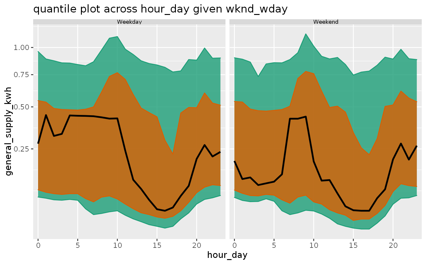
library(dplyr) library(ggplot2) smart_meter10 %>% filter(customer_id == "10017936") %>% gran_advice(gran1 = "wknd_wday", gran2 = "hour_day")#> The chosen granularities are harmonies #> #> Recommended plots are: violin lv quantile boxplot #> #> Number of observations are homogenous across facets #> #> Number of observations are homogenous within facets #> #> Cross tabulation of granularities : #> #> # A tibble: 24 x 3 #> hour_day Weekday Weekend #> <fct> <dbl> <dbl> #> 1 0 910 366 #> 2 1 908 366 #> 3 2 909 366 #> 4 3 910 366 #> 5 4 910 366 #> 6 5 910 366 #> 7 6 909 366 #> 8 7 908 366 #> 9 8 908 366 #> 10 9 908 366 #> # … with 14 more rows# choosing quantile plots from plot choices smart_meter10 %>% filter(customer_id == "10017936") %>% prob_plot( gran1 = "wknd_wday", gran2 = "hour_day", response = "general_supply_kwh", plot_type = "quantile", quantile_prob = c(0.1, 0.25, 0.5, 0.75, 0.9) ) + scale_y_sqrt()#>#>