Plotting probability distributions across granularities

Plot probability distribution of univariate series across bivariate temporal granularities.

prob_plot(
  .data,
  gran1 = NULL,
  gran2 = NULL,
  hierarchy_tbl = NULL,
  response = NULL,
  plot_type = NULL,
  quantile_prob = c(0.01, 0.1, 0.25, 0.5, 0.75, 0.9, 0.99),
  facet_h = NULL,
  symmetric = TRUE,
  alpha = 0.8,
  threshold_nobs = NULL,
  ...
)

Arguments

.data	a tsibble
gran1	the granularity which is to be placed across facets. Can be column names if required granularity already exists in the tsibble. For example, a column with public holidays which needs to be treated as granularity, can be included here.
gran2	the granularity to be placed across x-axis. Can be column names if required granularity already exists in the tsibble.
hierarchy_tbl	A hierarchy table specifying the hierarchy of units and their relationships.
response	response variable to be plotted.
plot_type	type of distribution plot. Options include "boxplot", "lv" (letter-value), "quantile", "ridge" or "violin".
quantile_prob	numeric vector of probabilities with value in [0,1] whose sample quantiles are wanted. Default is set to "decile" plot.
facet_h	levels of facet variable for which facetting is allowed while plotting bivariate temporal granularities.
symmetric	If TRUE, symmetic quantile area <- is drawn. If FALSE, only quantile lines are drawn instead of area. If TRUE, length of quantile_prob should be odd and ideally the quantile_prob should be a symmetric vector with median at the middle position.
alpha	level of transperancy for the quantile area
threshold_nobs	the minimum number of observations below which only points would be plotted
...	other arguments to be passed for customising the obtained ggplot object.

Value

a ggplot object which can be customised as usual.

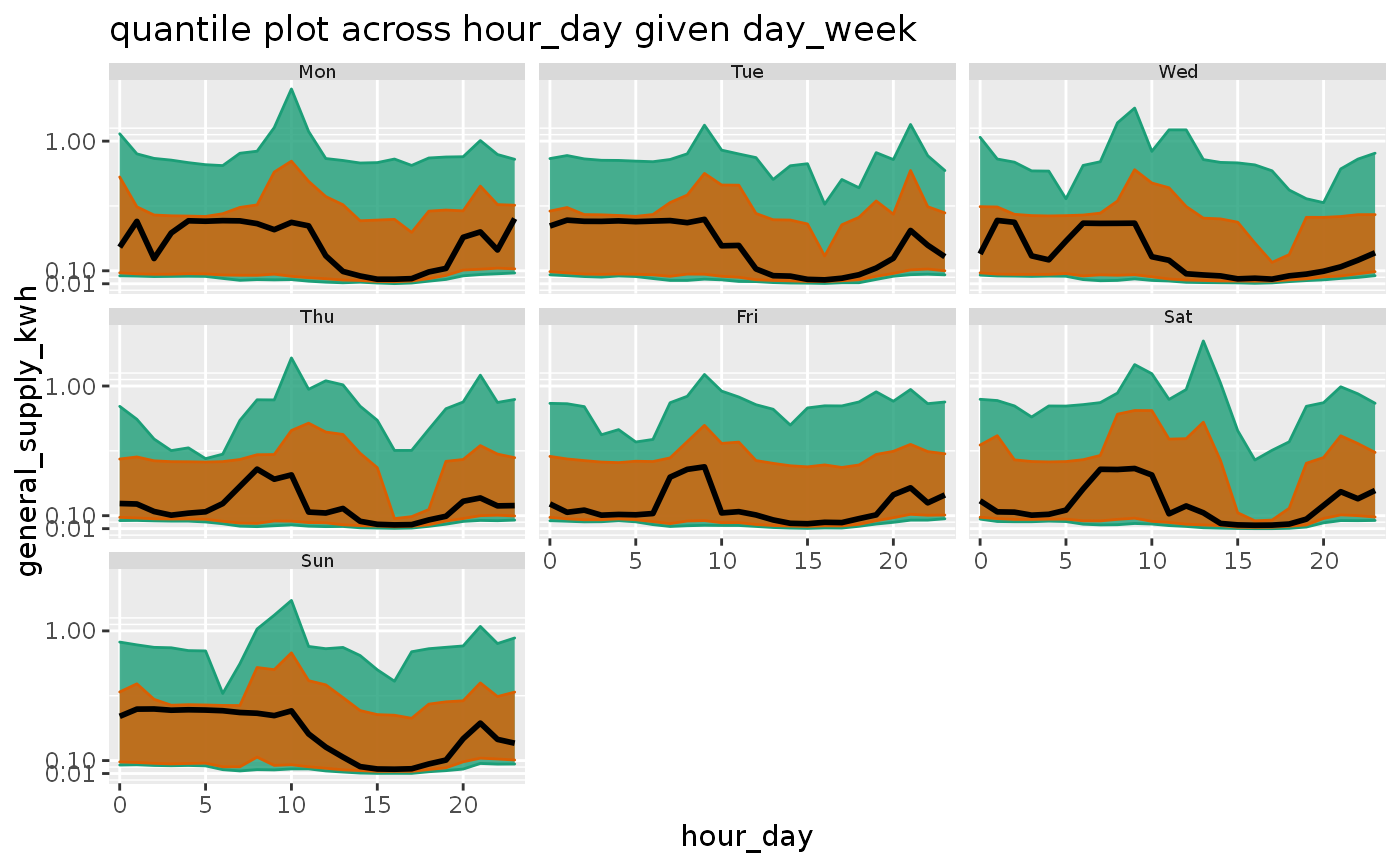
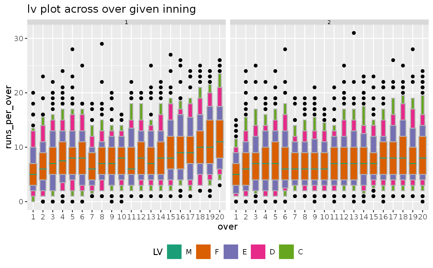
Examples

library(tsibbledata)
library(ggplot2)
library(tsibble)
library(lvplot)
library(dplyr)

smart_meter10 %>%
dplyr::filter(customer_id %in% c("10017936")) %>%
prob_plot(
  gran1 = "day_week", gran2 = "hour_day",
  response = "general_supply_kwh", plot_type = "quantile",
  quantile_prob = c(0.1, 0.25, 0.5, 0.75, 0.9),
  symmetric = TRUE,
   outlier.colour = "red",
  outlier.shape = 2, palette = "Dark2"
) + scale_y_continuous(breaks = c(0.01, 0.1, 1.00))
#> Joining, by = c("day_week", "hour_day")
#> Joining, by = c("day_week", "hour_day")


cricket_tsibble <- cricket %>%
  mutate(data_index = row_number()) %>%
  as_tsibble(index = data_index)

hierarchy_model <- tibble::tibble(
  units = c("index", "over", "inning", "match"),
  convert_fct = c(1, 20, 2, 1)
)

cricket_tsibble %>%
  prob_plot("inning", "over",
    hierarchy_tbl = hierarchy_model,
    response = "runs_per_over",
    plot_type = "lv"
  )
#> Joining, by = c("inning", "over")
#> Joining, by = c("inning", "over")